Why Rare Events Need More Than Just Data
An intuitive look at why rare events are difficult to emulate from limited data, and how local instability can provide the missing dynamical context.
Based on our NeurIPS 2026 oral paper
Mechanism-Aware Ensemble Conditioning for Data-Limited Emulation of Extreme Events
A model of a complex dynamical system may reproduce its frequently observed behavior with very small prediction error, while giving an inaccurate description of its most critical excursions. This distinction is particularly important for extreme events, whose low probability makes them difficult to represent in training data, even when their consequences are substantial.
Learning the bulk does not ensure accurate tails
Extreme events occur in natural, engineered, and economic systems. Examples include rogue ocean waves, heat waves, unusually large structural loads, cascading failures in power grids, and extreme financial losses. In a dynamical systems setting, such events are typically defined through an observable of the system, for example the wave height or the load acting on a structure, that exceeds a prescribed high threshold. Such systems may spend most of their time in a frequently visited regime and occasionally enter regions where finite-time amplification produces large excursions before the dynamics return to their usual behavior. Extreme values generally occupy the low-probability tails of the observable's distribution. [Sapsis, 2021] [Farazmand & Sapsis, 2019]
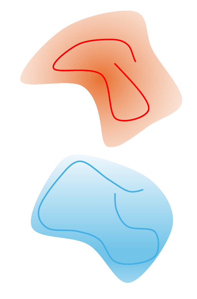
In our example, the training data come from two simulations of the same fluid flow. The high-resolution simulation is our reference and the cheaper coarse model simulation misses some small-scale motion. Those missing scales can affect extreme events even when the two simulations look similar most of the time. Generating a sufficiently long high-resolution trajectory to capture these rare extremes directly is prohibitively expensive.
This motivates the central question of our work: Can we extract and make use of more of the dynamical information already contained in the limited data available to us, rather than relying on increasingly expensive high-resolution simulations? Our theoretical contribution shows how a small ensemble of perturbed trajectories acts as a sensor of local finite-time instability. In this article, we illustrate how that information can be used in supervised learning to improve the long-time statistics of a coarsely simulated model, with particular emphasis on extreme events.
As a representative example, we consider a two-layer quasi-geostrophic (QG) flow. [Paper, Appendix C.1] Similarly, we have an expensive high-resolution reference and a cheaper coarsely resolved model. Before comparing these models, two difficulties need to be addressed. Their spatial resolutions differ, so we project the high-resolution state onto the coarse grid to express both in a common state space. Moreover, because the flow is chaotic, two freely evolving trajectories separate even when their initial conditions are close. A direct pointwise comparison would then mix the structural error of the coarse model with chaotic divergence of the trajectories, leaving the learning algorithm to fit this misalignment and noise instead of the unresolved dynamics. We therefore use nudging during training to keep the nudged-coarse trajectory in a neighborhood of the projected reference. [Paper, §2]
More details on nudging The equations for comparable training trajectories
Let the high-resolution state satisfy the evolution equation with vector field , and let denote the coarse-model vector field. We use to project the reference onto the coarse state space. The three relevant evolutions are the reference, the freely evolving coarse model, and the deterministically nudged coarse model.
Here the high-resolution state is denoted by , its projection by , the unconstrained coarse trajectory by , and the nudged trajectory by . The nudging timescale controls the strength of relaxation toward the projected reference and is chosen to balance two competing requirements: keeping the coarse trajectory sufficiently close to the reference while preserving the intrinsic dynamics and statistical characteristics of the coarse model's attractor. Projection makes the numerical states spatially comparable, while nudging reduces the effect of chaotic phase separation over the finite training interval. Neither operation supplies the missing fine-scale physics, and nudging is not itself the learned correction. [Paper, §2] [Paper, Appendix D]
One system, four views
Our objective with this QG example is to seek an inexpensive emulator that reproduces the long-time distribution of the reference, including the frequency and spatial extent of events with return periods longer than those observed during training.
01 / The idea
Using an ensemble to sense transient instability
When nearby trajectories separate rapidly, the flow is temporarily sensitive to small disturbances. Finite-time Lyapunov exponents, Cauchy–Green deformation tensors, and optimally time-dependent (OTD) modes provide well-established means of describing transient amplification. Their direct computation, however, requires the Jacobian, tangent-equation integrations, or additional evolution equations, which are computationally infeasible in high-dimensional settings. We instead apply small random perturbations to the nudged coarse model and track how the resulting trajectories spread.
In detail we evolve independent ensemble deviations driven by small stochastic perturbations. The ensemble members satisfy the following stochastic differential equation:
Here are independent Brownian motions, and is the noise intensity. The deterministic terms describe the nudged-coarse evolution, while the stochastic forcing continuously excites nearby directions. When these perturbations are small, the way the ensemble expands and contracts provides information about the local dynamics, rather than merely a measure of forecast uncertainty. [Paper, §2.2]
From two simulators to a local ensemble
How does this look in the QG data?
For the QG system considered here, the resulting ensemble is illustrated below. We show representative stochastically perturbed trajectories for different noise intensities, together with their deviations from the deterministically nudged coarse solution. These deviations provide information about the local response of the dynamics to small perturbations.
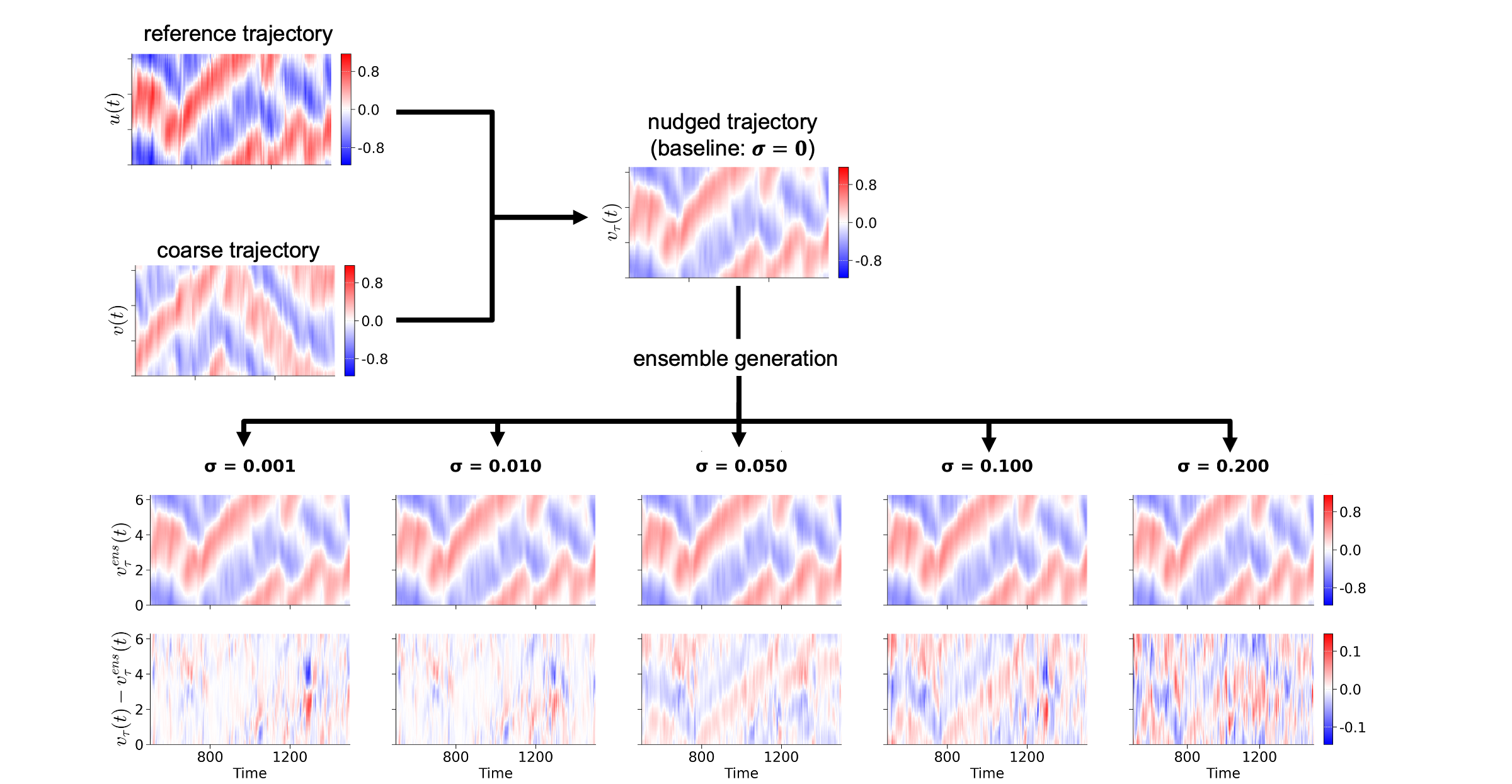
The important point is that the resulting ensemble spread is not arbitrary. Perturbations are damped along contracting directions and can grow in directions of finite-time instability, so the evolving distribution of nearby trajectories contains information about local deformation. We show mathematically that, in the small-noise regime, the ensemble covariance is governed by the same finite-time deformation kernels that characterize local amplification. This provides a dynamical interpretation of the ensemble as a non-intrusive instability sensor.
The mathematical connection Covariance evolution, assumptions, and finite-ensemble guarantees
We denote by the ensemble mean and define the covariance of the centered fluctuations as
Here, denotes a solution of the stochastic ensemble equation. The covariance characterizes both the magnitude and the directional structure of the ensemble spread.
Linearizing the drift of the stochastic ensemble around its mean gives a matrix Lyapunov equation, perturbed by a remainder that accounts for the nonlinear terms.
The linearized operator is evaluated along the mean perturbed coarse state and includes the stabilizing contribution from nudging.
The terms involving describe the local stretching and contraction of the ensemble, while the isotropic forcing injects perturbations continuously. On a fixed finite interval, this relation requires the stated smoothness conditions and second- and fourth-moment bounds on the deviations. The small-noise bounds have the following scaling.
Under these bounds and the stated regularity conditions, the covariance remainder is of order as increases.
Let be the fundamental solution of the linearized nudged dynamics. Integrating the covariance equation gives
The covariance therefore combines the deformation of the initial spread with deformation accumulated from the stochastic forcing over the interval. These kernels contain the same local stretching information used in finite-time instability analysis, although their time integral is not identical to a single Cauchy–Green tensor. Relating their leading subspaces further requires separation of the relevant growth directions.
For a finite ensemble of independent centered samples, Theorem 2.2 quantifies the error in the estimated leading covariance subspace. If the fourth moment is bounded by and the relevant eigenvalues are separated by a gap , the expected projector error is bounded by . This is a finite-sample statement about the inferred geometry, not a theorem asserting that all rare-event statistics can be recovered from a short dataset. [Paper, §2.2] [Paper, Appendix A]
02 / The method
An instability signal for existing learning architectures
The ensemble provides information about the local dynamics, but this information becomes useful for emulation only when the learning algorithm can respond to it. An important feature of our framework is that the conditioning is independent of the particular neural-network backbone. Instead of replacing an established corrector or redesigning its internal architecture, we introduce a small interface that makes the ensemble-derived dynamical context available to its existing hidden features.
For this purpose we use feature-wise linear modulation (FiLM) [Perez et al., 2018].
The FiLM implementationBackbone agnostic introduction of dynamical context
A small conditioning network transforms the dynamical context into scale and shift coefficients, which modulate the hidden representation of the original model. If is a hidden feature vector and is the ensemble-derived context, the modulation takes the form
The coefficients depend on the instantaneous dynamical context, so the learned corrector can adapt its internal response when the flow enters a sensitive regime. This is a lightweight addition to an existing learning pipeline rather than a new dynamical model. In our comparisons we retain the original backbones and baseline training setups, including their architecture and hyperparameter choices, and learn the additional conditioning within the supervised training procedure. [Paper, §2.3]
Projection and nudging provide comparable training states.
Ensemble response supplies dynamical context.
Learn context-dependent gains and offsets without replacing the corrector.
We demonstrate this interface on different types of neural-network models, including a Transformer-style residual-attention corrector and a probabilistic recurrent STORN model. Improvements in both settings show that the conditioning is not specific to a particular backbone architecture. We compare each conditioned model with its unconditioned counterpart, keeping the underlying backbone, its hyperparameters, and the baseline training setup the same. This makes the effect of the added dynamical context easier to assess. [Paper, §3] [Paper, §4]
The following animation shows for the QG example how this FiLM context is introduced into the existing STORN pipeline.
Building FiLM-STORN, one stage at a time
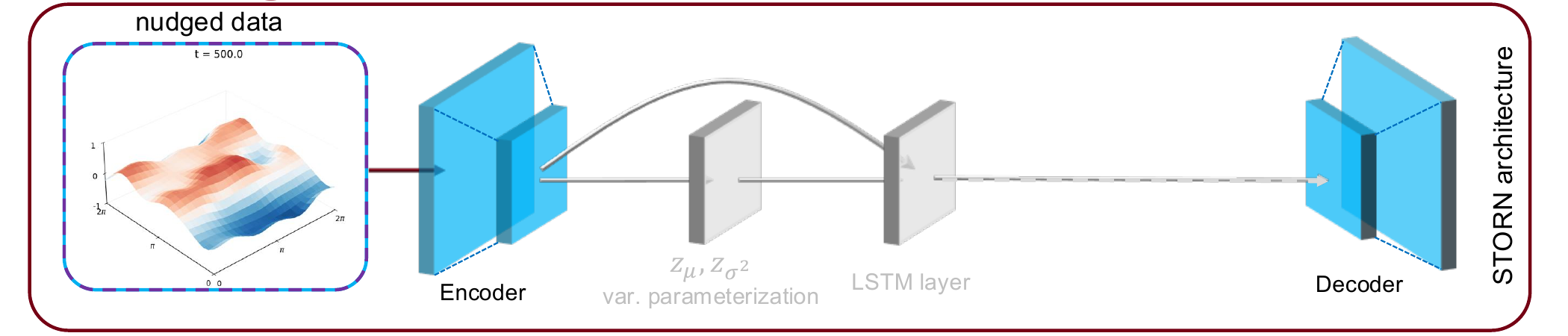
During long-time deployment, the QG corrector uses statistics of the freely evolving coarse trajectory as an approximate context signal. This is a deliberate choice that ensures the method operates independently of the high-resolution reference. While generating the nudged ensemble during training requires reference data, neither nudging nor additional reference information is needed at deployment. The corrected coarse simulation can therefore be evaluated over arbitrarily long horizons without introducing information from the reference trajectory into the correction process. [Paper, Appendix D]
03 / The results
Extreme-event statistics beyond the training horizon
We examine the sensing mechanism in a low-dimensional chaotic system, where independent OTD modes provide a characterization of transient instability. The leading ensemble-covariance direction becomes active during the same instability episodes as the OTD mode, supporting the interpretation of stochastic ensemble spread as a probe of finite-time amplification. [Paper, §3]
For the QG flow the high-resolution reference is generated on a 128 × 128 grid and the coarse model evolves on a 24 × 24 grid. In the strongly data-limited experiment, our FiLM-conditioned model is trained on just 50 time units of nudged-coarse and high-resolution reference data and a few-member ensemble. This is a particularly restrictive setting because the training trajectory is short even for characterizing the bulk of the distribution dynamics, while extreme events with long return periods may not occur within the training horizon at all. This places us in a substantially more data-limited regime than previously demonstrated for successful correction of the same QG system. Earlier work found that approximately 500 to 1,000 time units were necessary to reproduce the relevant long-time statistics accurately. [Barthel Sorensen et al., 2024] [Barthel Sorensen et al., 2026] With only 50 time units, the available record is therefore insufficient not only for resolving extremes but also for providing a well-sampled representation of the frequently visited dynamics.
We then evaluate the corrected model for 50,000 time units, a horizon 1,000 times longer than the training length . The purpose is to determine whether the learned model reproduces the reference distribution, including events whose characteristic return times are much longer than the duration of its training data. The reference simulation over the evaluation interval is used to construct the benchmark statistics and is not supplied to the deployed corrector.
We compare against an unconditioned STORN trained on the same 50-unit record and a second unconditioned STORN trained on 1,000 time units of high-resolution data, which represents the state-of-the-art in this literature [Barthel Sorensen et al., 2024] [Barthel Sorensen et al., 2026]. Alongside the overall probability density, we examine the frequency of high-threshold exceedances and the spatial area affected by these events. These two diagnostics are important because accurate bulk statistics alone do not establish that the model reproduces how frequently extreme episodes occur or how extensively they develop within the flow. [Paper, §4]
How often do extremes occur?
Mean absolute error in the probability that the field’s magnitude exceeds a high threshold somewhere in the domain, averaged over both layers and three extreme thresholds.
Absolute frequency error · lower is better
About 41% less frequency error than the baseline trained on the same 50 time units, and about 39% less than the baseline trained on 1,000.
See every value and its source
| Method | Training horizon | Frequency error | Area error | Log-density error | KL |
|---|---|---|---|---|---|
| STORN | 50 | 0.12118 | 0.01574 | 11.970 | 0.07079 |
| FiLM-STORN | 50 | 0.07199 | 0.01047 | 8.2959 | 0.03646 |
| STORN | 1,000 | 0.11726 | 0.01195 | 5.3454 | 0.00393 |
With the same short training record, ensemble conditioning improves all four reported diagnostic errors relative to the unconditioned model. More strikingly, even with just 50 time units of training data, the conditioned model has lower average errors for how often high-threshold events occur and how much area they cover than the baseline trained on 1,000 time units. The longer-trained baseline remains better on the overall KL divergence and log-density errors. These results are expected as both the KL-divergence and log-density are dominated by the frequently observed dynamics, which are better represented in a longer training record. The interactive comparison above shows the results reported in Table 2.
This result also motivates the computational comparison. Generating the perturbed ensemble requires additional coarse simulations, but their cost is small relative to extending an expensive high-resolution reference from 50 to 1,000 time units. Importantly, we find that only a small ensemble is needed to obtain substantial improvements. The results presented here use just a two-member ensemble. The conditioned approach therefore achieves more accurate averaged high-threshold statistics using substantially less high-resolution supervision and a much shorter training trajectory. In this regime, enriching the training information with a description of the dynamics can be more effective than obtaining many more examples of the same frequently observed behavior.
The big take-away is that local dynamical information can be extracted from inexpensive numerical trajectories and supplied to existing learning architectures without redesigning the underlying numerical solver or neural-network backbone. The effectiveness of the approach ultimately depends on the quality of the underlying coarse model. Although the coarse dynamics need not reproduce the reference accurately, they must retain the essential dynamical structures and amplification mechanisms of the original system. If these mechanisms are absent or fundamentally misrepresented, the ensemble cannot recover the missing information through perturbations alone. [Paper, §5]
When high-resolution data are limited, the response of a stochastically evolved ensemble can provide valuable information about extreme-event mechanisms that is not contained in the observed trajectory alone.
If this connects with a system you work on, I would love to hear about it. For questions, possible applications, or a more detailed presentation, get in touch.
Conversation around the paper
If LinkedIn blocks the embedded preview in your browser, read the original post directly.