Angular momentum (QM)

Consider a spherical potential in 3D. We see that the Schrödinger equation in 3D is in terms of the Laplacian. In spherical coordinates it takes the form

\begin{align*} \nabla^2 &= \frac{1}{r^2} \frac{\partial}{\partial r} \left(r^2 \frac{\partial}{\partial r}\right) + \frac{1}{r^2\sin\theta} \frac{\partial}{\partial \theta}\left(\sin\theta \frac{\partial}{\partial \theta}\right) + \frac{1}{r^2 \sin^2\theta} \left(\frac{\partial^2}{\partial \phi^2}\right) \\ &= \frac{\partial^2}{\partial r^2} + \frac{2}{r} \frac{\partial}{\partial r} + \frac{1}{r^2} \left(\frac{\partial^2}{\partial \theta^2} + \cot\theta\frac{\partial}{\partial\theta} + \frac{1}{\sin^2\theta}\frac{\partial^2}{\partial\phi^2}\right). \end{align*}

We define an operator $\LL$ which will be associated with angular momentum

\begin{align*} \LL^2 &= -\hbar^2 \left(\frac{\partial^2}{\partial \theta^2} + \cot\theta\frac{\partial}{\partial\theta} + \frac{1}{\sin^2\theta}\frac{\partial^2}{\partial\phi^2}\right) \\ \nabla^2 &= \frac{\partial^2}{\partial r^2} + \frac{2}{r}\frac{\partial}{\partial r} - \frac{\LL^2}{\hbar^2r^2}. \end{align*}

This gives us the Schrödinger equation

-\frac{\hbar^2}{2m} \left[ \frac{\partial^2}{\partial r^2} + \frac{2}{r}\frac{\partial}{\partial r} - \frac{\LL^2}{\hbar^2r^2} \right] \psi(\rr) + V(r) \psi(\rr) = E\psi(\rr).

Since we assume the potential is spherical, we guess that there exists a separable solution $\psi(r,\theta,\phi) = R(r) Y(\theta,\phi)$ . This gives us

\begin{align*} \left[ -\frac{\hbar^2}{2m} \left(\frac{\partial}{\partial r^2} + \frac{2}{r}\frac{\partial}{\partial r}\right) + V(r)\right] R(r)Y(\theta,\phi) + \frac{L^2}{2mr^2}R(r)Y(\theta,\phi) = ER(r)Y(\theta,\phi) \end{align*}

Divide by $R(r)Y(\theta,\phi)$ , we see that since the two terms depend on different variables, they can only equal a constnat $E$ if they are both constants.

\begin{align*} \frac{1}{R(r)} \left[-\frac{\hbar^2}{2m}\left(\frac{\partial}{\partial r^2} + \frac{2}{r}\frac{\partial}{\partial r}\right) + V(r)\right] R(r) + \frac{\constant}{2mr^2} = E. \end{align*}

\begin{align*} \frac{\LL^2}{2mr^2}Y(\theta,\phi) &= \frac{\constant}{2mr^2}Y(\theta,\phi) =: E_L(r) Y(\theta,\phi) \\ \LL^2 Y(\theta,\phi) &= 2mr^2E_L(r)Y(\theta,\phi). \end{align*}

We see $Y$ is an eigenvector of $\LL^2$ and $2mr^2E_L(r)$ is its eigenvalue.

The angular momentum operator $\LL = \xx \times \pp$ (TODO: proof). The components are $\LL_x = yp_z - zp_y$ , etc.

Before we continue, consider the commutators of the relevant operators.

\begin{align*} [\LL_x,\LL_y] &= [yp_z-zp_y,zp_x-xp_z] = y[p_z,z]p_x + x[z,p_y]p_y \\ &= \frac{\hbar}{i}yp_x + i\hbar xp_y=i\hbar(xp_y-yp_x) \\ &= i\hbar \LL_z \\ [\LL_y,\LL_z] &= i\hbar \LL_x \\ [\LL_z,\LL_x] &= i\hbar \LL_y. \end{align*}

We see that two angular momentum components commute only if the third is zero, so it may seem like we can measure two components exactly (i.e. that $\LL_x,\LL_y$ have some simultaneous eigenstates). However, in order for that to be possible all components need to commute, and for any two to commute the third must be zero. We see that exactly measuring any two components is only possible if all three are zero.

\begin{align*} [\LL_z,\LL^2] &= [\LL_z,\LL_x^2] + [\LL_z,\LL_y^2] = \LL_x[\LL_z,\LL_x] + [\LL_z,\LL_x]\LL_x + \LL_y[\LL_z,\LL_y] + [\LL_z,\LL_y]\LL_y \\ &= i\hbar \LL_x\LL_y + i\hbar \LL_y\LL_x - i\hbar\LL_y\LL_x - i\hbar\LL_x\LL_y = 0. \end{align*}

We can, however, have simultaneous eigenstates of $\LL^2$ and $\LL_z$ . We denote an eigenstate $\ket{l,m}$ such that

\begin{align*} \LL_z\ket{l,m} &= m\hbar\ket{l,m} \\ \LL^2\ket{l,m} &= \hbar^2l(l+1)\ket{l,m}. \end{align*}

Here $m$ is called the azimuth or magnetic quantum number, and $l$ is called the quantum number of total momentum. By convention we consider $\LL_z$ instead of one of the other components.

We define raising and lowering operators $\LL_\pm = \LL_x\pm i\LL_y$ . Since they are Hermitian, $\LL_+\adj = \LL_-$ and vice-versa. The commutator relationships are

\begin{align*} [\LL^2,\LL_\pm] &= 0 \\ [\LL_\pm,\LL_z] &= \mp \hbar \LL_\pm. \end{align*}

What does $\LL_\pm$ do to $\ket{l,m}$ ?

\begin{align*} [\LL^2,\LL_\pm] &= 0 \implies \LL_\pm\ket{l,m} \text{ has } \LL^2 \text{ eigenvalue } l \\ \LL_z ( \LL_+ \ket{l,m} ) &= (\LL_+\LL_z + \hbar \LL_+)\ket{l,m} \\ &= \LL_+(m+1)\hbar \ket{l,m} \\ \LL_+\ket{l,m} &\propto \ket{l,m+1} \\ \text{similarly } \LL_-\ket{l,m} &\propto \ket{l,m-1}. \end{align*}

Now define $\ket{l,\widetilde{m+1}} := \LL_+\ket{l,m}$ and consider the norm

\begin{align*} |\ket{l,\widetilde{m+1}}|^2 &= \braket{l,\widetilde{m+1}|l,\widetilde{m+1}} = \braket{\LL_+(l,m) | \LL_+(l,m)} \\ &= \braket{l,m|\LL_+\adj \LL_+ | l,m} = \braket{l,m|\LL_-\LL_+|l,m} \\ \LL_-\LL_+ &= (\LL_x-i\LL_y)(\LL_x+i\LL_y) \\ &= \LL_x^2 \LL_y^2 + i(\LL_x\LL_y - \LL_y\LL_x) \\ &= \LL_x^2 + \LL_y^2 - \hbar\LL_z \tag{from the commutator} \\ &= \LL^2 - \LL_z^2 - \hbar\LL_z \\ \braket{l,m | \LL_-\LL_+ | l,m} &= \big[l(l+1) - m(m+1)\big] \hbar^2 \end{align*}

Since $\braket{l,m | \LL_-\LL_+ | l,m}$ is a squared magnitude, $\big[l(l+1) - m(m+1)\big] \hbar^2 \ge 0$ . This means $m \le l$ . We can do the same for $\LL_-$ to find $m \ge -l$ . This is an important conclusion:

\begin{align*} -l \le m \le l. \end{align*}

Since $\LL_+$ transforms a $-l$ eigenstate to an $l$ eigenstate in integer steps, $l$ must be an integer or a ½-integer. We will see that integer eigenstates correspond to orbital angular momentum, while ½ eigenstates correspond to spin.

Spherical harmonics

We call $Y_l^m(\theta,\phi)$ the spacial wavefunction for $\ket{l,m}$ . From the properties of the operators we showed above, we see

\begin{align*} \LL_z Y_l^m(\theta,\phi) &= m\hbar Y_l^m(\theta,\phi) = \frac{\hbar}{i}\frac{\d}{\d\phi} Y_l^m(\theta,\phi) \\ Y_l^m(\theta,\phi) &= e^{im\phi} P_{lm}(\theta) \\ \LL_+Y_l^l(\theta,\phi) &= 0 \\ &= \hbar e^{i\phi} \left(\frac{\d}{\d\phi} + i\cot\theta\frac{\d}{\d\phi}\right) e^{il\phi} P_l^l(\theta) \\ &= \left(\frac{\d}{\d\theta} - l\cot\theta\right) e^{i(l+1)\phi} P_l^l(\theta) \\ P_l^l(\theta) &= C_l^l \sin^l\theta \\ Y_l^l(\theta,\phi) &= C_l^l \sin^l\theta e^{il\phi}. \end{align*}

Since we have $Y_l^l$ we can reach any other $Y_l^m$ by using the raising and lowering operators we found above. The family of functions $Y_l^m$ are called the spherical harmonics.

Some rules of thumb for spherical harmonics:

The $\phi$ dependence is always $e^{im\phi}$ .
The $\theta$ dependence is a polynomial of $\cos$ and $\sin$ of degree $l$ .

Geometric interpretation

\begin{align*} \braket{l,l|\LL^2|l,l} &= \hbar^2l(l+1) \\ \braket{l,l|\LL_z^2|l,l} &= \hbar^2 l^2. \end{align*}

We see that $\LL^2 > \LL_z^2$ even in the maximum $m$ state, which tells us that angular momentum can never be fully lined up in one axis. Meanwhile, we see that

\begin{align*} \braket{\LL_x^2} &= \frac14 \braket{l,l|(\LL_+-\LL_-)^2|l,l} = \frac14 \braket{l,l | \LL_+^2 - \LL_+\LL_- - \LL_-\LL_+ + \LL_-^2 | l,l} \\ &= \frac12 \braket{l,l | \LL^2 - \LL_z^2 | l,l} = \frac12 \big(\hbar^2 l(l+1) - \hbar^2 l^2\big) \\ \braket{\LL_x^2} = \braket{\LL_y^2} &= \frac l2 \hbar^2 \text{ for } \ket{l,l}. \end{align*}

This makes sense by the uncertainty principle.

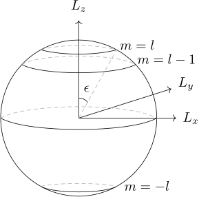
The sphere below shows a geometric interpretation of this phenomenon. The radius of the sphere is $\LL^2$ , and the rings show (in this case) the possible $\LL_z$ . They are drawn about the $z$ axis here, but could just as well be shown along any axis. The highest possible ring, at $m=l$ , is still below the top of the sphere, leaving some component of $\LL$ in the $x$ and $y$ direction.

The angle $\epsilon \to 0$ as $l \gg 1$ , which is why in the classical limit angular momentum appears fully localized in one direction.

Electron angular magnetic dipole moment

The magnetic dipole moment of an electron resulting from its angular momentum can be written as

\begin{align*} \vec\mu_e = -g_l \mu_B \frac{\vec L}{\hbar} \end{align*}

where $g_l = 1$ . A similar formula can be used to find the spin dipole moment of an electron.