1182

Rapid, Time-Resolved Brain Imaging with Multiple Clinical Contrasts using Wave-Shuffling.

Siddharth Srinivasan Iyer^1,2, Daniel Polak^1,3,4, Congyu Liao¹, Steve Cauley¹, Berkin Bilgic¹, and Kawin Setsompop¹

¹Athinoula A. Martinos Center for Biomedical Imaging, Charlestown, MA, United States, ²Department of Electrical Engineering and Computer Science, Massachusetts Institute of Technology, Cambridge, MA, United States, ³Department of Physics and Astronomy, Heidelberg University, Heidelberg, Germany, ⁴Siemens Healthcare GmbH, Erlangen, Germany

Synopsis

Previously, we presented Wave-Shuffling: a technique that combines random-sampling and the temporal low-rank priors of T₂-shuffling with the sinusoidal gradients of Wave-CAIPI to achieve highly-accelerated, time-resolved acquisitions. In this work, we optimize and apply Wave-Shuffling to T₂-SPACE and MPRAGE to achieve rapid, 1 mm-isotropic resolution, time-resolved imaging of the brain where we recover a time-series of clinical contrast. We also present preliminary explorations into Joint-Contrast Wave-Shuffling to boost signal-to-noise ratio and reconstruction-conditioning at high accelerations.

Introduction

Previously, we presented Wave-Shuffling: a technique that combines random-sampling and the temporal low-rank priors of $T_2-$ shuffling¹ with the sinusoidal gradients of Wave-CAIPI² to achieve highly-accelerated, time-resolved acquisitions. In this work, we optimize and apply Wave-Shuffling to $T_2-$ SPACE and MPRAGE to achieve rapid, $1 mm-$ isotropic resolution, time-resolved imaging of the brain where we recover a time-series of clinical contrast. We also present preliminary explorations into Joint-Contrast Wave-Shuffling to boost signal-to-noise ratio and reconstruction-conditioning at high accelerations.

Wave-Shuffling Model And Reconstruction

Forward Model. A succinct description of Wave-Shuffling is as follows:

b = \underset{≜ A}{\underset{⏟}{M F_{y z} W F_{x} R E Φ}} c,

$b=\underbrace{MF_{yz}WF_{x}RE \Phi}_{\triangleq A}\;c,$ where

c

$c$ represents the underlying temporal coefficients from the Shuffling model,

Φ

$\Phi$ is the temporal basis that expands the coefficients to a model-based time-series of images,

E

$E$ is the ESPIRiT³ operator,

R

$R$ is the readout

(x)

$(x)$ resize operator to a larger FOV to account for the readout alias-spreading as a function of spatial phase-encode positions

(y, z)

$(y, z)$ induced by Wave-CAIPI,

F

$F$ is the Fourier Transform,

W

$W$ is the Wave-CAIPI Point Spread Function (PSF),

M

$M$ is the phase-encode sampling mask, and

b

$b$ is the acquired data.

Reconstruction. The reconstruction problem is posed as follows:

c^{*} = \underset{c}{a r g m i n} \frac{1}{2} | | A c - b | |_{2}^{2} + λ | | T (c) | |_{1},

$c^*=\underset{c}{\mathrm{argmin}}\;\frac{1}{2}||Ac-b||_2^2+\lambda||T(c)||_1,$ where

T

$T$ is the spatial Wavelet transform and

λ

$\lambda$ is the regularization. This problem is solved with BART⁴ using FISTA⁵.

Methods

A healthy subject was scanned on a 3T scanner using 32-channel head coil with $\;T_2-$ SPACE and MPRAGE sequences that were modified to play sinusoidal gradients during readout and randomly reorder phase-encode sampling. The matrix size for both cases were $256\times256\times256$ at $1mm$ isotropic.

MPRAGE. Fully-sampled (randomly ordered) data with and without sinusoidal readout gradients was acquired using $TI=1.2s,TR=2.5s,$ flip angle of $8^\circ,T_{\text{acquisition}}=11\;\text{minutes}$ and an echo-train length of $256$ . The data was retrospectively under sampled to contain $100\%,50\%,25\%$ of the possible $256\times256$ phase-encode points, which we denote $R1,R2,R4$ respectively.

$T_2-$ SPACE. Fully-sampled (randomly ordered) data with $89\%\;$ Partial Fourier (PF) in the $\;y\;$ direction, was acquired with a variable flip angle train⁶ of echo-train length of $\;196$ , echo spacing of $\;4.6ms$ . $TR=3.2s,T_{\text{acquisition}}=16\;\text{minutes}$ and sinusoidal gradients. The data was retrospectively under sampled to contain $25\%$ of the possible $228\times256\;$ phase-encode points ( $22\%$ of $256\times256$ ), which we denote $R4$ . PF was accounted for by applying homodyne projection-onto-convex-sets (POCS) to the reconstructed coefficients.

Wave Parameter Optimization. Through simulations, it was observed that larger readout alias-spreading provides better reconstruction conditioning. This spreading is proportional to the maximum amplitude of the sinusoidal gradient, which is maximized by minimizing the number of cycles given gradient-slew and readout duration limitations. In our previous work⁷, we showed that small cycles create large corkscrew k-space trajectories that result in signal mixing across partition-encoding due to $T_1/T_2\;$ recovery over the acquisition-train, which causes ringing artifacts in standard wave-CAIPI. The Shuffling model resolves signal-recovery over time, allowing for small cycles without artifacts. Consequently, for $\;T_2-$ SPACE, we used $\;2\;$ cycles with a gradient maximum-amplitude of $25mT/m$ . For MPRAGE with a lower readout bandwidth, $\;8\;$ cycles with a gradient maximum-amplitude of $16mT/m$ was used for good conditioning while avoiding artifacts of lower-cycle cases with undesirable velocity-encoding.

Results

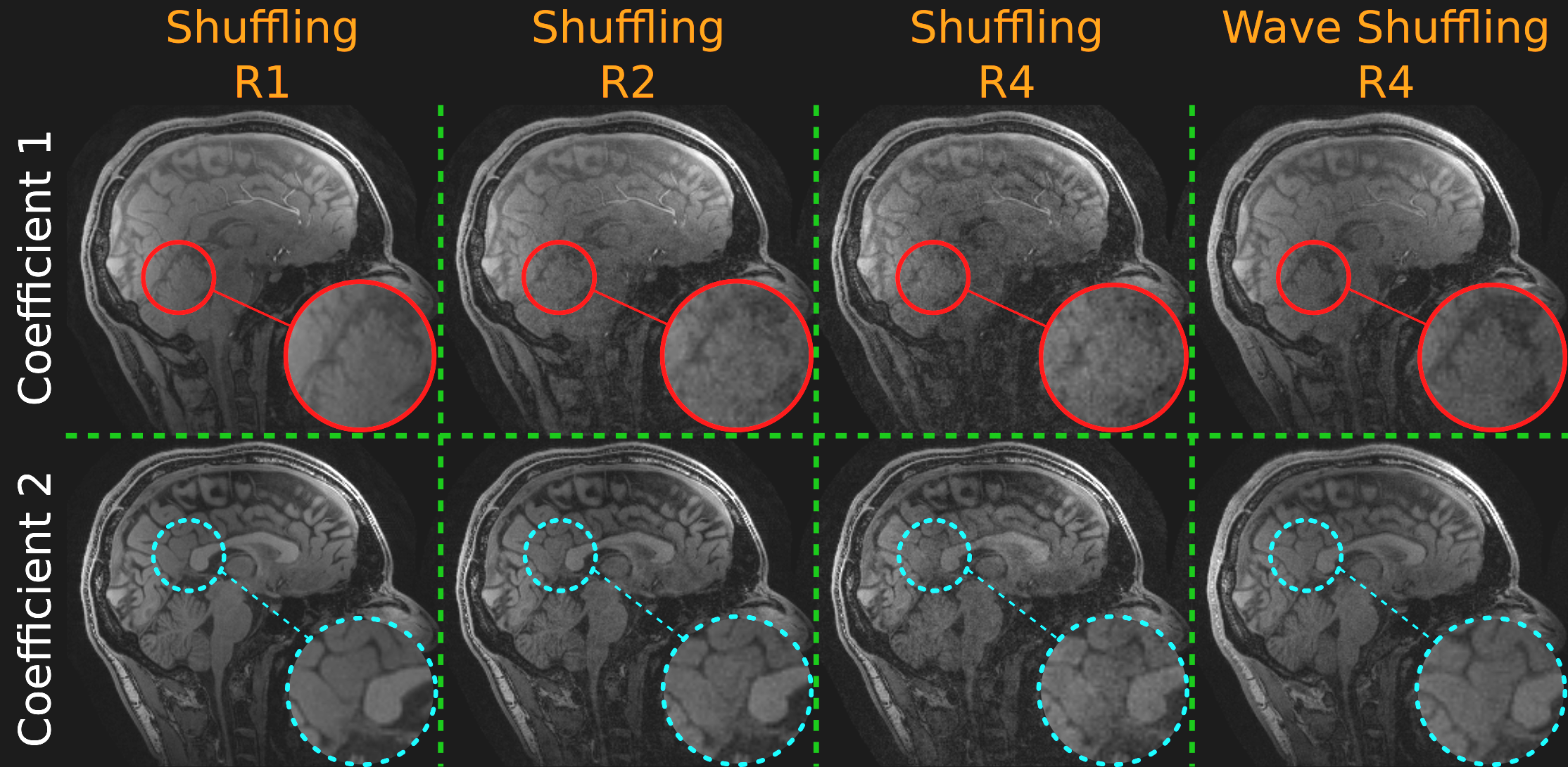
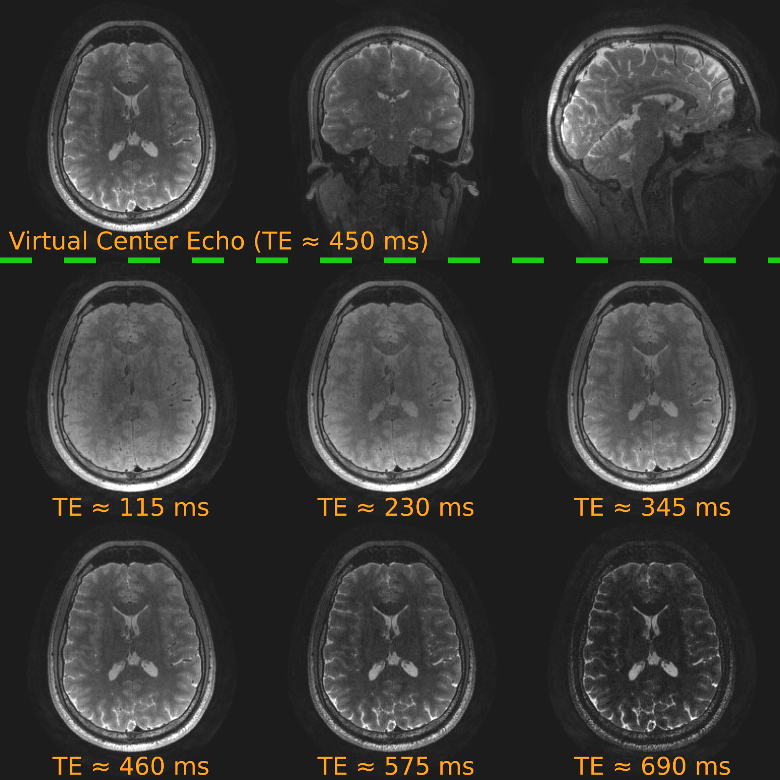
Figure 1 shows that Shuffling without Wave-CAIPI provides clean reconstruction at

R 1

$R1$ with increased noise at

R 2

$R2$ and artifacts at

R 4

$R4$ . Wave-Shuffling achieves clean results at

R 4

$R4$ and more closely resembles Shuffling

R 1

$R1$ upto noise considerations. Figure

2

$2$ demonstrates Wave-Shuffling's ability to recover a sharp image of the clinical

T_{2} -

$T_2-$ SPACE contrast at

R 4

$R4$ , which is the virtual echo at the center of the echo-train (top-panel), as well as the time-series of signal evolution (bottom-panel). Figure

3

$3$ is an animated GIF that shows the signal-evolution from Wave-Shuffling of

R 4

$R4$ MPRAGE and

R 4 T_{2} -

$R4\;T_2-$ SPACE.

Joint Contrast Considerations

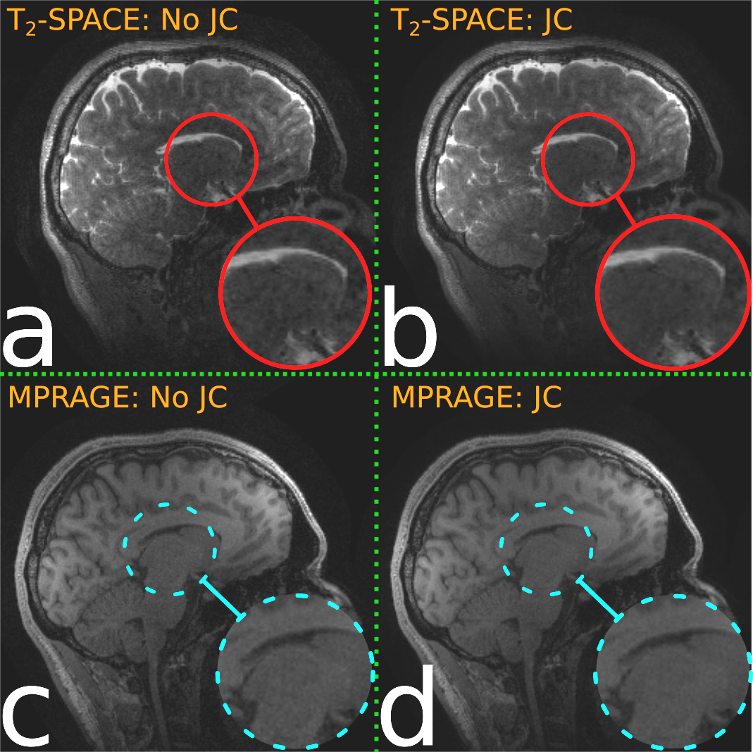
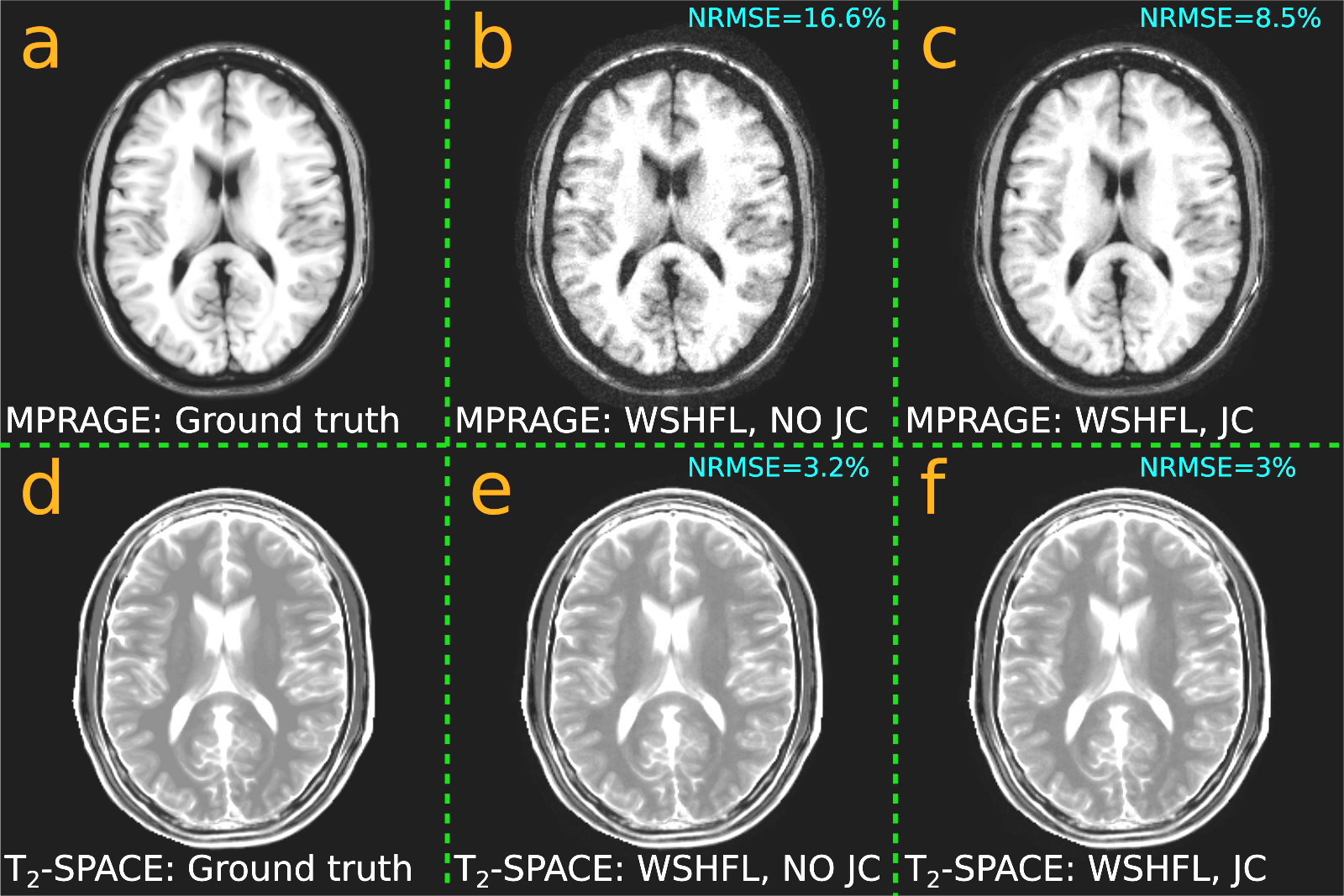
Given recent developments of joint reconstruction for multi-contrast acquisitions^8-11, we present our preliminary explorations of Joint-Contrast Wave-Shuffling. The magnitude coefficients of the above reconstructed $R4$ MPRAGE and $R4\;T_2$ -SPACE data are registered with respect to each other using FSL¹² (since the same subject was scanned on different sessions), and a locally low-rank threshold is applied to promote structural similarities. The result is depicted in Figure 4, where the prior is seen to help remove visual noise with a marginal improvement to normalized root mean squared error with respect to the respective $R1$ magnitude coefficients.

We plan to explore this direction further by incorporating the different signal evolution of MPRAGE and $T_2-$ SPACE into $\Phi$ so as to enforce joint-contrast with the data-consistency term. Simulation results of the same are presented in Figure 5. Brain web¹³ phantom courtesy of Dr. Bo Zhao.

Conclusion

We successfully optimized and applied Wave-Shuffling to

T_{2} -

$T_2-$ SPACE and MPRAGE to provide fast, time-resolved imaging with clinical contrasts at

3 T

$3T$ . Preliminary results using Joint-Contrast was also presented, which helps de-noise reconstruction at high accelerations.

Acknowledgements

This work was supported in part by NIH research grants: R01MH116173, R01EB020613,R01EB019437, U01EB025162, P41EB015896, and the shared instrumentation grants: S10RR023401, S10RR019307, S10RR019254, S10RR023043.

References

Tamir, J.I., Uecker, M., Chen, W., Lai, P., Alley, M.T., Vasanawala, S.S. and Lustig, M., 2017. T2 shuffling: Sharp, multicontrast, volumetric fast spin‐echo imaging. Magnetic resonance in medicine, 77(1), pp.180-195.
Bilgic, B., Gagoski, B.A., Cauley, S.F., Fan, A.P., Polimeni, J.R., Grant, P.E., Wald, L.L. and Setsompop, K., 2015. Wave‐CAIPI for highly accelerated 3D imaging. Magnetic resonance in medicine, 73(6), pp.2152-2162.
Uecker, M., Lai, P., Murphy, M.J., Virtue, P., Elad, M., Pauly, J.M., Vasanawala, S.S. and Lustig, M., 2014. ESPIRiT—an eigenvalue approach to autocalibrating parallel MRI: where SENSE meets GRAPPA. Magnetic resonance in medicine, 71(3), pp.990-1001.
Uecker, M., 2018. Mrirecon/Bart. Latest version located at https://github.com/mrirecon/bart.
Beck, A. and Teboulle, M., 2009. A fast iterative shrinkage-thresholding algorithm for linear inverse problems. SIAM journal on imaging sciences, 2(1), pp.183-202.
Mugler, J.P., Kiefer, B. and Brookeman, J.R., 2000, April. Three-dimensional T2-weighted imaging of the brain using very long spin-echo trains. In Proceedings of the 8th Annual Meeting of ISMRM (p. 687).
Polak, D., Setsompop, K., Cauley, S., Gagoski,B., Batt, H., Maier. F., Wald, L., and Bilgic, B., 2017. Wave-CAIPI for Highly Accelerated MP-RAGE Imaging. International Society for Magnetic Resonance in Medicine, 25th Scientific Meeting, Hawaii, USA.
Bilgic, B., Kim, T.H., Liao, C., Manhard, M.K., Wald, L.L., Haldar, J.P. and Setsompop, K., 2018. Improving parallel imaging by jointly reconstructing multi‐contrast data. Magnetic resonance in medicine, 80(2), pp.619-632.
Kilic, T., Ilicak, E., Çukur, T. and Saritas, E., 2017. Improved SPIRiT Operator for Joint Reconstruction of Multiple T2-Weighted Images. International Society for Magnetic Resonance in Medicine, 25th Scientific Meeting, Hawaii, USA, p. 5165.
Bilgic, B., Cauley, S.F., Wald, L.L. and Setsompop, K., 2018. Joint SENSE Reconstruction for Faster Multi-Contrast Wave Encoding. International Society for Magnetic Resonance in Medicine 27th Scientific Meeting, Paris, France, p. 940.
Tamir, J., Taviani, V., Vasanawala, S. and Lustig, M., 2017. T1-T2 Shuffling: Multi-Contrast 3D Fast Spin-Echo with T1 and T2 Sensitivity. International Society for Magnetic Resonance in Medicine, 25th Scientific Meeting, Hawaii, USA.
Jenkinson, M., Beckmann, C.F., Behrens, T.E., Woolrich, M.W. and Smith, S.M., 2012. Fsl. Neuroimage, 62(2), pp.782-790.
Collins, D., Zijdenbos, A., Kollokian, V., Sled, J., Kabani, N., Holmes, C. and Evans, A., 1998. Design and construction of a realistic digital brain phantom. IEEE Trans. Med. Imaging, vol. 17, pp. 463–468.

Figures

Figure 1. Comparing Shuffling without and with Wave-CAIPI sinusoidal gradients for MPRAGE. Shuffling without Wave-CAIPI provides clean reconstruction at

R 1

$R1$ with increased noise at

R 2

$R2$ and artifacts at

R 4

$R4$ . Wave-Shuffling achieves clean results at

R 4

$R4$ and more closely resembles Shuffling

R 1

$R1$ upto noise considerations. Additionally, the Normalized Root Mean Squared (NRMSE) of

R 4

$R4$ Shuffling compared to

R 1

$R1$ Shuffling is

29.38 %

$29.38\%$ versus

13.71 %

$13.71\%$ between

R 4

$R4$ Wave-Shuffling compared to

R 1

$R1$ Wave-Shuffling.

Figure 2. Demonstrating Wave-Shuffling applied to

T_{2} -

$T_2-$ SPACE with

\approx 22 %

$\approx 22\%$ phase encode points acquired. The first row shows Wave-Shuffling's ability to recover a sharp image of the clinical

T_{2} -

$T_2-$ SPACE contrast, which is the virtual echo at the center of the echo-train. The rest of the image demonstrates Wave-Shuffling's ability to time-resolve and recover temporal evolution of the signal.

Figure 3. (Compressed Animated GIF) First row depicts orthogonal slices from

R 4

$R4$ MPRAGE as it evolves through the time-series as reconstructed by Wave-Shuffling.

25 %

$25\%$ encode points were used. Second row depicts orthogonal slices from "

R 4

$R4$ "

T_{2} -

$T_2-$ SPACE as it evolves through the time-series as reconstructed by Wave-Shuffling.

\approx 22 %

$\approx 22\%$ encode points were used.

Figure 4. Joint Contrast (JC). Magnitude coefficients of reconstructed data are registered to each other and locally-lowrank (LLR) is applied across coefficients. (a) is an MPRAGE

R 4

$R4$ Wave-Shuffling coefficient after reconstruction and (b) is the same after the JC-LLR. (c) is a

T_{2} -

$\;T_2-$ SPACE

R 4

$\;R4$ Wave-Shuffling coefficient after reconstruction and (d) is the same after the JC-LLR. JC is seen to help remove visual noise.

Figure 5. Joint Contrast (JC) through data-consistency. All the images are the respective virtual echos at the center of their echo-trains. (a) Ground truth MPRAGE. (b) MPRAGE Wave-Shuffling without JC. (NRMSE

= 16.6 %

$=16.6\%$ ) (c) MPRAGE Wave-Shuffling with JC. (NRMSE

= 8.5 %

$=8.5\%$ ) (d) Ground truth

T_{2} -

$T_2-$ SPACE. (e)

T_{2} -

$T_2-$ SPACE Wave-Shuffling without JC. (NRMSE

= 3.2 %

$=3.2\%$ ) (f)

T_{2} -

$T_2-$ SPACE Wave-Shuffling with JC. (NRMSE

= 3 %

$=3\%$ ). JC as data-consistency is seen to improve the MPRAGE reconstruction.

Proc. Intl. Soc. Mag. Reson. Med. 27 (2019)

1182