This course covers vector and multi-variable calculus. At MIT it is labeled 18.02 and is the second semester in the MIT freshman calculus sequence. Topics include vectors and matrices, parametric curves, partial derivatives, double and triple integrals, and vector calculus in 2- and 3-space.

As its name suggests, multivariable calculus is the extension of calculus to more than one variable. That is, in single variable calculus you study functions of a single independent variable

y=f(x).

In multivariable calculus we study functions of two or more independent variables, e.g.,

z=f(x, y) or w=f(x, y, z).

These functions are interesting in their own right, but they are also essential for describing the physical world.

Many things depend on more than one independent variable. Here are just a few:

1. In thermodynamics pressure depends on volume and temperature.
2. In electricity and magnetism, the magnetic and electric fields are functions of the three space variables (x,y,z) and one time variable t.
3. In economics, functions can depend on a large number of independent variables, e.g., a manufacturer's cost might depend on the prices of 27 different commodities.
4. In modeling fluid or heat flow the velocity field depends on position and time.

Single variable calculus is a highly geometric subject and multivariable calculus is the same, maybe even more so. In your calculus class you studied the graphs of functions y=f(x) and learned to relate derivatives and integrals to these graphs. In this course we will also study graphs and relate them to derivatives and integrals. One key difference is that more variables means more geometric dimensions. This makes visualization of graphs both harder and more rewarding and useful.

By the end of the course you will know how to differentiate and integrate functions of several variables. In single variable calculus the Fundamental Theorem of Calculus relates derivatives to integrals. We will see something similar in multivariable calculus and the capstone to the course will be the three theorems (Green's, Stokes' and Gauss') that do this.

After completing this course, students should have developed a clear understanding of the fundamental concepts of multivariable calculus and a range of skills allowing them to work effectively with the concepts.

The basic concepts are:

1. Derivatives as rates of change, computed as a limit of ratios
2. Integrals as a 'sum,' computed as a limit of Riemann sums

The skills include:

1. Fluency with vector operations, including vector proofs and the ability to translate back and forth among the various ways to describe geometric properties, namely, in pictures, in words, in vector notation, and in coordinate notation.
2. Fluency with matrix algebra, including the ability to put systems of linear equation in matrix format and solve them using matrix multiplication and the matrix inverse.
3. An understanding of a parametric curve as a trajectory described by a position vector; the ability to find parametric equations of a curve and to compute its velocity and acceleration vectors.
4. A comprehensive understanding of the gradient, including its relationship to level curves (or surfaces), directional derivatives, and linear approximation.
5. The ability to compute derivatives using the chain rule or total differentials.
6. The ability to set up and solve optimization problems involving several variables, with or without constraints.
7. An understanding of line integrals for work and flux, surface integrals for flux, general surface integrals and volume integrals. Also, an understanding of the physical interpretation of these integrals.
8. The ability to set up and compute multiple integrals in rectangular, polar, cylindrical and spherical coordinates.
9. The ability to change variables in multiple integrals.
10. An understanding of the major theorems (Green's, Stokes', Gauss') of the course and of some physical applications of these theorems.

This course, designed for independent study, has been organized to follow the sequence of topics covered in an MIT course on Multivariable Calculus. The content is organized into four major units:

1. Vectors and Matrices
2. Partial Derivatives
3. Double Integrals and Line Integrals in the Plane
4. Triple Integrals and Surface Integrals in 3-Space

Each unit has been further divided into parts (A, B, C, etc.), with each part containing a sequence of sessions. Because each session builds on knowledge from previous sessions, it is important to progress through the sessions in order. Each session covers an amount you might expect to complete in one sitting.

Within each unit you will be presented with sets of problems at strategic points, so you can test your understanding of the material. At the end of each unit, there is a comprehensive exam that covers all of the topics you learned in the unit.

MIT expects its students to spend about 150 hours on this course. More than half of that time is spent preparing for class and doing assignments. It’s difficult to estimate how long it will take you to complete the course, but you can probably expect to spend an hour or more working through each individual session.

This unit covers the basic concepts and language we will use throughout the course. Just like every other topic we cover, we can view vectors and matrices algebraically and geometrically. It is important that you learn both viewpoints and the relationship between them.

Vectors are basic to this course. We will learn to manipulate them algebraically and geometrically. They will help us simplify the statements of problems and theorems and to find solutions and proofs.

Determinants measure volumes and areas. They will also be important in part B when we use matrices to solve systems of equations.

The basic point of this part is to formulate systems of linear equations in terms of matrices. We can then view them as analogous to an equation like 7x = 5.

In order to use them in systems of equations we will need to learn the algebra of matrices; in particular, how to multiply them and how to find their inverses.

Geometrically, a linear equation in x, y and z is the equation of a plane. Solving a system of linear equations is equivalent to finding the intersection of the corresponding planes.

Parametric equations define trajectories in space or in the plane. Very often we can think of the trajectory as that of a particle moving through space and the parameter as time. In this case, the parametric curve is written (x(t); y(t); z(t)), which gives the position of the particle at time t.

A moving particle also has a velocity and acceleration. These are vectors which vary in time. We will learn to compute them as derivatives of the position vector.

In this unit we will learn about derivatives of functions of several variables. Conceptually these derivatives are similar to those for functions of a single variable.

1. They measure rates of change.
2. They are used in approximation formulas.
3. They help identify local maxima and minima.

As you learn about partial derivatives you should keep the first point, that all derivatives measure rates of change, firmly in mind. Said differently, derivatives are limits of ratios. For example,

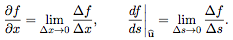
Of course, we’ll explain what the pieces of each of these ratios represent.

Although conceptually similar to derivatives of a single variable, the uses, rules and equations for multivariable derivatives can be more complicated. To help us understand and organize everything our two main tools will be the tangent approximation formula and the gradient vector.

Our main application in this unit will be solving optimization problems, that is, solving problems about finding maxima and minima. We will do this in both unconstrained and constrained settings.

We start this unit by learning to visualize functions of several variables using graphs and level curves. Following this we will study partial derivatives. These will be used in the tangent approximation formula, which is one of the keys to multivariable calculus. It ties together the geometric and algebraic sides of the subject and is the higher dimensional analog of the equation for the tangent line found in single variable calculus. We will use it in part B to develop the chain rule.

We will apply our understanding of partial derivatives to solving unconstrained optimization problems. (In part C we will solve constrained optimization problems.)

As in single variable calculus, there is a multivariable chain rule. The version with several variables is more complicated and we will use the tangent approximation and total differentials to help understand and organize it.

Also related to the tangent approximation formula is the gradient of a function. The gradient is one of the key concepts in multivariable calculus. It is a vector field, so it allows us to use vector techniques to study functions of several variables. Geometrically, it is perpendicular to the level curves or surfaces and represents the direction of most rapid change of the function. Analytically, it holds all the rate information for the function and can be used to compute the rate of change in any direction.

In this part we will study a new type of optimization problem: that of finding the maximum (or minimum) value of a function w = f(x, y, z) when we are only allowed to consider points (x, y, z) which are constrained to lie on a surface. The technique we will use to solve these problems is called Lagrange multipliers.

This unit starts our study of integration of functions of several variables. To keep the visualization difficulties to a minimum we will only look at functions of two variables. (We will look at functions of three variables in the next unit.)

Our main objects of study will be two types of integrals:

1. Double integrals, which are integrals over planar regions.
2. Line or path integrals, which are integrals over curves.

All integrals can be thought of as a sum, technically a limit of Riemann sums, and these will be no exception. If you make sure you master this simple idea then you will find the applications and proofs involving these integrals to be straightforward.

We will conclude the unit by learning Green's theorem which relates the two types of integrals and is a generalization of the Fundamental Theorem of Calculus. Along the way we will introduce the concepts of work and two dimensional flux and also two types of derivatives of vector valued functions of two variables, the curl and the divergence.

In part A, we will learn about double integration over regions in the plane. Conceptually an integral is a sum. We will apply this idea to computing the mass, center of mass and moment of inertia of a two dimensional body and the volume of a region bounded by surfaces.

In order to compute double integrals we will have to describe regions in the plane in terms of the equations describing their boundary curves. After that, the computation just becomes two single variable integrations done iteratively.

A vector field attaches a vector to each point. For example, the sun has a gravitational field, which gives its gravitational attraction at each point in space. The field does work as it moves a mass along a curve. We will learn to express this work as a line integral and to compute its value.

In physics, some force fields conserve energy. Such conservative fields are determined by their potential energy functions. We will define what a conservative field is mathematically and learn to identify them and find their potential function.

In this part we will learn Green's theorem, which relates line integrals over a closed path to a double integral over the region enclosed. The line integral involves a vector field and the double integral involves derivatives (either div or curl, we will learn both) of the vector field.

First we will give Green's theorem in work form. The line integral in question is the work done by the vector field. The double integral uses the curl of the vector field. Then we will study the line integral for flux of a field across a curve. Finally we will give Green's theorem in flux form. This relates the line integral for flux with the divergence of the vector field.

In our last unit we move up from two to three dimensions. Now we will have three main objects of study:

1. Triple integrals over solid regions of space.
2. Surface integrals over a 2D surface in space.
3. Line integrals over a curve in space.

As before, the integrals can be thought of as sums and we will use this idea in applications and proofs.

We'll see that there are analogs for both forms of Green's theorem. The work form will become Stokes' theorem and the flux form will become the divergence theorem (also known as Gauss' theorem). To state these theorems we will need to learn the 3D versions of div and curl.

In this part we will learn to compute triple integrals over regions in space. We will learn to do this in three natural coordinate systems: rectangular, cylindrical and spherical.

Here we will extend Green's theorem in flux form to the divergence (or Gauss') theorem relating the flux of a vector field through a closed surface to a triple integral over the region it encloses. Before learning this theorem we will have to discuss the surface integrals, flux through a surface and the divergence of a vector field.

In this part we will extend Green's theorem in work form to Stokes' theorem. For a given vector field, this relates the field's work integral over a closed space curve with the flux integral of the field's curl over any surface that has that curve as its boundary.