
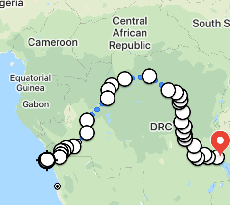
Frogs on the island of São Tomé seem to have an odd history. The island is only 13 million years old, yet it is inhabited by frogs unlike any others in the vicinity. Genetic analysis shows that all sampled São Tomé frogs have are remarkably similar to frogs found in Tanzania (at the Kibebe farm), Uganda (at Lake Victoria), and at Kenya (specifically, Mt. Kenya). These are all in East Africa, while São Tomé is a small island off the West African coast (Figure 1).
How many frogs would we expect to arrive at São Tomé, drifting from East Africa to the West African coast and to the island?
Similarly to a Feynman path integral, the probability of a frog reaching the island is given by summing over all its possible paths. However, in street-fighting style, we only consider here the largest contributing path. A flood in Lake Tanganyika, where such frogs are found, would send frogs down the Lukuga River and onto the Congo River, which swiftly drains into the Atlantic Ocean. Because my everyday experience does not stretch quite as far as Lake Tanganyika (someone should organize a conference there!), this problem will require a few more papers than usual; nevertheless, we will be sure to swashbuckle our way through order-of-magnitude estimations!
As we shall see later, the treacherous conditions on the path to São Tomé require many frogs to complete the Congo River journey. Hence, we will begin by considering only the largest possible floods. Although the annual wet season brings sufficient rainfall to raise the water level of Lake Tanganyika, P. nilotica have almost certainly evolved to migrate accordingly and avoid being swept up by currents. In particular, P. nilotica are grass frogs, suggesting that they do not live directly on the shoreline and will be naturally selected to move away from fast-moving water during periods of rapid (but seasonal) rainfall.
Lake Tanganyika has a shoreline of almost 2000 km. Since the lake is extremely large and likely lacks well-defined currents (especially during floods), we will require that a frog must live near the Lukuga River to wash down the Congo River. If we assume that you can find a P. nilotica every 10 m\(^2\) (which is surprisingly a conservative frog density estimate [1]), we can expect around 100,000 frogs per square kilometer. Since frogs require moisture to breathe through their skin, it is likely that in the wet season frogs will live up to several kilometers from the shoreline in the wet season, especially considering that P. nilotica are found further away from bodies of water, such as Kibebe Farms.
The Lukuga River changes direction seasonally and with longer-term climate changes, and it is the only river that drains Lake Tanganyika. When the lake water level is low (typically in the dry season), the Lukuga River is only a narrow creek that is blocked before reaching the Congo River. During the wet season, however, the Lukuga River serves as a major outlet of water from Lake Tanganyika. Again, to consider the largest exoduses of frogs, we’re only interested in the largest floods of Lake Tanganyika.
Explorers in the 19th century observed Lake Tanganyika and left historical records detailing the surrounding environment. In the 1870s, the lake level was seen to steeply increase during a period of excessive rainfall, taking about 1 km of additional shore during the dry season [4]. A more detailed analysis of sediment cores show that the lake achieved unusually high levels three times in the last 2500 years: 500 AD, 1500 AD, and 1870 AD [5]. This suggests that large floods occur roughly every 800 years, yielding a total of 16,000 large floods over the last 13 million years. If we consider the frogs along 5 km on either side of the Lukuga River and 5 km north and south of the river’s connection to Lake Tanganyika with a 1 km depth corresponding to flooding, a total of 20 km\(^2\) or 2,000,000 frogs can be endangered by the floods and find themselves travelling down the Lukuga.
When the explorer Verney Lovett Cameron visited Lake Tanganyika in 1874, he found that after journeying four or five miles down the Lukuga River “navigation was rendered impossible owing to the masses of floating vegetation” [4]. This implies that rafts were plentiful for frogs! Natives suggested that Cameron “cut passages for canoes,” which indicates that the water surface was at least 25% covered in vegetation. If 2,000,000 frogs are randomly dropped on the water surface, we would then expect 500,000 frogs to land on rafts. These frogs are then sent down the Lukuga River at a rate of 1 to 1.5 knots (as observed by Cameron), i.e., around 2 km/h.
The Lukuga River merges with the Congo River and flows to the Atlantic Ocean over the course of 3000 km, as measured at a resolution of around 50 km (Figure 1, right). Of course, the river curves along its path; currents are more likely to push frogs in individual directions at a resolution of 0.5 km than 50 km. A river has a fractal dimension of around 1.06 to 1.2 as measured in an Australian study [6], so we take an average of about \(D=1.1\). The length \(L\) of a path measured with a ruler of length \(R\) is given by $$\begin{aligned} L &= c R^{1-D}, \end{aligned}$$ where \(c\) is a constant. Solving for \(c=4400\) with our measured data, we find that \(R = 0.5\) km gives a distance of \(L = 4800\) km. (This is slightly longer than the Wikipedia-worthy length of the Congo River connecting to Lake Tanganyika, measuring 4400 km.) Thus, the frogs will likely journey a distance of 4800 km day and night, taking a total of around 200 days to reach the Atlantic Ocean.
Out of the 500,000 frogs that start this journey, relatively few will see the ocean. Some frogs will die peacefully of old age, since the average lifetime of a frog is around 10 years (as we previously observed); however, this barely changes the order of magnitude, and thus we ignore it. The most prevalent cause of departure would likely be rafts swerving off course and running into the river bank. However, the Congo flows very quickly and is very wide, typically ranging from around 5 to 10 km in width throughout its course. Additionally, since the volume flow rate of the river must be constant (\(A_1v_1=A_2v_2\)) to prevent water from accumulating or depleting from river regions, we can expect that the rafts will have a larger downstream velocity component when the river becomes narrower. Thus, we estimate that perhaps 1% of the frogs will run into the shore every 10 km. Starting with 500,000 frogs, we conclude that \((500,000\;\mathrm{frogs})(0.99)^{480} \approx 4000\) frogs will exit the Atlantic Ocean.
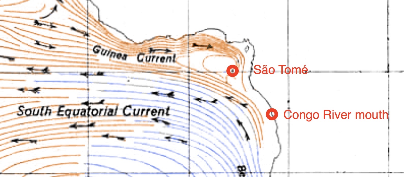
Upon leaving the Congo River, the frogs must follow either the South Equatorial Current into the Guinea current onto western São Tomé or take the warm South Equatorial Current directly to their destination (Figure 2, left). Just like electric field lines, the density of ocean current streamlines scales with current strength. From the figure, we estimate that the warm South Equatorial Current is twice as strong as the cold South Equatorial Current, implying that around 2/3 of the rafts head towards São Tomé instead of South America.
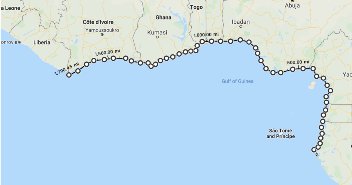
If it successfully finds the warm South Equatorial Current, a frog will continue to drift until it hits coastline. São Tomé has a total of 209 km of shore compared to around 2,700 km of West African shore (Figure 2, right). As in scattering cross-sections, the Guinea Current only sees half of São Tomé, so we estimate that around \(100/2700 \approx 4\%\) of the Guinea Current results in landfall on São Tomé. This is likely an underestimate, since the ocean current map shows streamlines curling away from the coast and towards São Tomé; additionally, they run parallel to much of the West African coast that we measured. Looking at the cross-sectional length of the coastline from the perspective of the Guinea Current, we probably overestimated its length by a factor of two, yielding a São Tomé landfall probability of 7%. Multiplying by 2/3, we find that around \(5\%\) of all rafts leaving the Congo River finds their way up the warm South Equatorial Current and back down the Guinea Current to São Tomé.
Another possible route indicated by the current map is to travel up the warm South Equatorial Current and directly change direction towards São Tomé. Only one of the five warm current streamlines point towards São Tomé and it is weaker, so we estimate that 10% of rafts will take this route instead of moving to the Guinea Current. If you take this narrow streamline, you would either make landfall in São Tomé or the land directly east of it, yielding a coast ratio of around \(100/700 \approx 14\%\). Again multiplying by \(2/3\), we have a probability of around \(9\%\).
Ocean currents typically move at a few miles per hour, or around 4-8 km/h. Going up the South Equatorial Current and down the Guinea Current is around 4000 km (20-30 days), while going directly to São Tomé is around 1000 km (5-7 days). During this time, the freshwater frogs are exposed to saltwater, which dehydrates them and reduces the survival rate. Indeed, the Xenopus laevis (which also lives along the Congo River) in 100% seawater can only survive for less than an hour [7].
This suggests that a frog must be able to remain largely dry (which also decreases its survival rate, although Xenopus laevis are known to survive for long periods of time in the absence of water). If we assume that the raft must be firm enough for the frog to stand on without being submerged in seawater — which is likely, since the raft has survived all the way down the Congo River, but to be conservative we estimate a probability of 50% — then the frog may be exposed to seawater around 10-30% of the time due to splashing. The paper notes that all frogs exposed to salinities below 25% seawater survived. However, they were also exposed to 75% freshwater to maintain moisture. Given that 35% seawater resulted in an average lifetime of around 40 hours but 25% seawater resulted in no harm, we estimate a characteristic survival duration of \(\tau=4\) days, where the probability of surviving after \(t\) days is given by \(e^{-t/\tau}\).
After 5-7 days, we have a survival rate of around 20-30%; after 20-30 days, we have a survival rate of around 1%. Adding all the two possible routes to São Tomé, we find that a P. nilotica leaving the Congo River mouth will arrive alive with probability $$\begin{aligned} (0.9)(0.05)(0.01) + (0.1)(0.09)(0.25) \approx 3\times 10^{-3}. \end{aligned}$$
For each of 16,000 floods over the last 13 million years, we expect 4000 frogs to (accidentally) attempt to colonize São Tomé, with a total of around 200,000 P. nilotica frogs landing on the island over its history, appearing in groups of 12 on average. However, most of these frogs would perish, since they would be unlikely to find a mate on the 209 km coastline!
To successfully breed and begin a colony, let us assume that we require at least 30 frogs to land on the island in a single flood. From the binomial theorem, the probability of this happening after \(f\) floods is $$\begin{aligned} P(\mathrm{success}) &= 1 - \left[1 - \sum_{k=m}^{n} \begin{pmatrix}n \\ k\end{pmatrix}p^k(1-p)^{n-k}\right]^f. \end{aligned}$$ Plugging in, \(p=3\times10^{-3}\), \(m=30\), \(n=4,000\), and \(f=16,000\), we find that \(P(\mathrm{success}) \approx 0.1\). Note that this result is sensitive to the number of frogs that are required to start a population. If we require 12 frogs to land at once, the probability of success is almost identically 1.
Hence, it makes sense to consider only the largest possible floods, since a smaller frog exodus is extremely unlikely to result in a sufficient number of frogs leaving the continent. Indeed, a study of Lake Tanganyika’s water level over the last 40,000 years shows even more dramatic fluctuations in the water level [8], indicating that floods larger than the 1870 flood we analyzed may have occurred. If we assume that the frog population initially affected by the flood has a standard deviation of 20% (i.e., convolving our estimate with a Gaussian), the probability of success (i.e., at least 30 frogs landing at once) increases to 0.96!
Under the assumption that 30 frogs landing on the island will always start a population, we conclude that an expected number of 15 (since \(0.96^{15} \approx 0.5\)) migrations will succeed. With logarithmic estimation uncertainty like \(\pm 1\) in base \(e\), 5 to 40 successful migrations will breed over the last 13 million years on the island.
An alternative (and cuter) analysis is the birthday problem. As we mentioned above, we expect an average of 12 frogs to land for each of 16,000 flood migrations (which is admittedly unnecessarily precise, but that is largely irrelevant for the upcoming computations). The coastline is about 200 km, and we require a male and female to find each other. Mating calls can be heard up to a kilometer away in some frog species (pg. 1349 of [9]), but since that is an upper limit we will take half the value (500 m) for the distance of P. nilotica mating calls. Assuming we need two pairs of frogs to find each other on the island, we can require that at least two males and two females land in the space of 2 km (each 500 m apart from each other). The birthday problem of finding k people in a room of \(n\) people with the same birthday can be estimated by a Poisson approximation $$\begin{aligned} P(\text{at least }k\text{ people with the same birthday in a room of \(n\) people}) &= 1 - \exp\left[\begin{pmatrix}n\\k\end{pmatrix}/365^{k-1}\right]. \end{aligned}$$ In our case, we want four frogs within a single “bucket” of 2 km, for a total of 100 buckets on the 200 km coastline of São Tomé: $$\begin{aligned} P(\text{at least }4\text{ out of 12 frogs within 2 km on the São Tomé coastline}) &= 1 - \exp\left[\begin{pmatrix}12\\4\end{pmatrix}/100^3\right]. \end{aligned}$$ For 16,000 floods over 13 million years, the expected number of successful migrations (defined to be when 4 frogs land within 2 km of each other) is given by the mean of the binomial distribution, multiplied by the probability of getting 2 male and 2 female, i.e., $$\begin{aligned} \frac{\begin{pmatrix}4\\2\end{pmatrix}}{2^4}(16,000)\left(1 - \exp\left[\begin{pmatrix}12\\4\end{pmatrix}/100^3\right]\right) \approx 3. \end{aligned}$$ This is undercounting due to the fact that the frogs would have on average 3-5 years to find each other on the island (undergoing a random walk), but it is overcounting due to the fact that the frogs may not breed successfully despite finding each other. Hence, we conclude with logarithmic uncertainty \(\pm 1\) in base \(e\) that 1 to 10 successful migrations will breed.