Fixed point/Linear stability analysis

In an autonomous (time-independent) ODE like

\dot x = f(x(t))

the fixed points are $x_*$ such that $f(x_*)=0$ .

We can examine the behavior of the ODE near a fixed point

\begin{align*} x(t) &= x_* + \epsilon(t) \\ \dot x &= \dot\epsilon. \end{align*}

We Taylor expand the equation and take the first nonzero term using the fact that $f(x_*)=0$ to find

\begin{align*} f(x) = f(x_* + \epsilon) &= f(x_*) + f'(x_*)\epsilon + \cdots \\ &= f'(x_*)\epsilon. \end{align*}

Then we call the linearized ODE $\dot\epsilon = \lambda\epsilon$ where $\lambda = f'(x_*)$ . The solution to this linearized ODE is $\epsilon(t) = \epsilon(0) e^{\lambda t}$ . We can understand the stability of a fixed point by looking at its linearized solution

If $f'(x_*) > 0$ then $x_*$ is linearly unstable, so perturbations of $\epsilon$ grow over time.
If $f'(x_*) < 0$ , then $x_*$ is linearly stable, so perturbations of $\epsilon$ decay over time.

Consider a slope field of $\dot y = (1-\frac{1}{4}y)y$ , an example of logistic growth.

We see there are two fixed points, $y_* = \{0,4\}$ (these are the nullclines of the ODE). Near $y=4$ , the derivative arrows point towards the fixed point, indicating that it is stable. Conversely, the derivatives point away from fixed point $y=0$ , indicating that it is unstable.

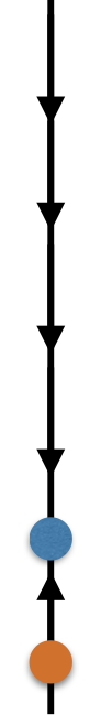
Phase space

The phase space/phase line of an autonomous ODE shows the stability around the fixed points. The figure below shows the phase line for the same logistic growth model as above.