Data visualization with R study guide
General structure
Overview The general structure of the code that is used to plot figures is as follows:
ggplot(...) +             # Initialization
  geom_function(...) +    # Main plot(s)
  facet_function(...) +   # Facets (optional)
  labs(...) +             # Legend (optional)
  scale_function(...) +   # Scales (optional)
  theme_function(...)     # Theme (optional)
We note the following points:
- The
ggplot()layer is mandatory. - When the
dataargument is specified inside theggplot()function, it is used as default in the following layers that compose the plot command, unless otherwise specified. - In order for features of a data frame to be used in a plot, they need to be specified inside the
aes()function.
Basic plots The main basic plots are summarized in the table below:
| Type | Command and parameters | Illustration |
| Scatter plot | geom_point( x, y, params ) | 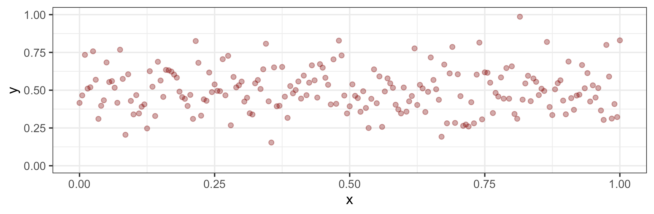 |
| Line plot | geom_line( x, y, params ) | 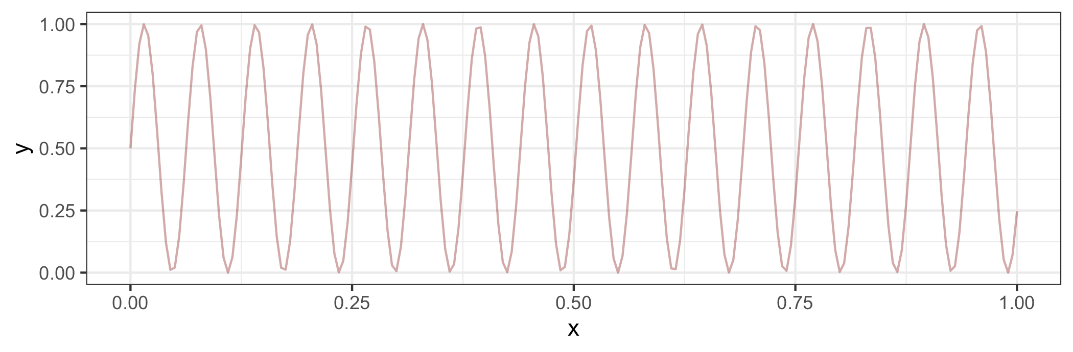 |
| Bar chart Histogram | geom_bar( x, y, params ) | 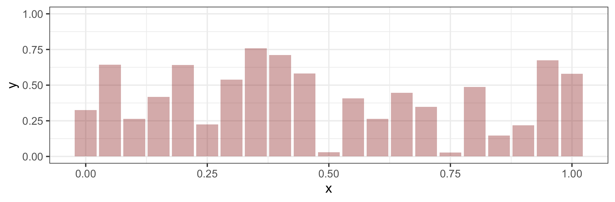 |
| Box plot | geom_boxplot( x, y, params ) | 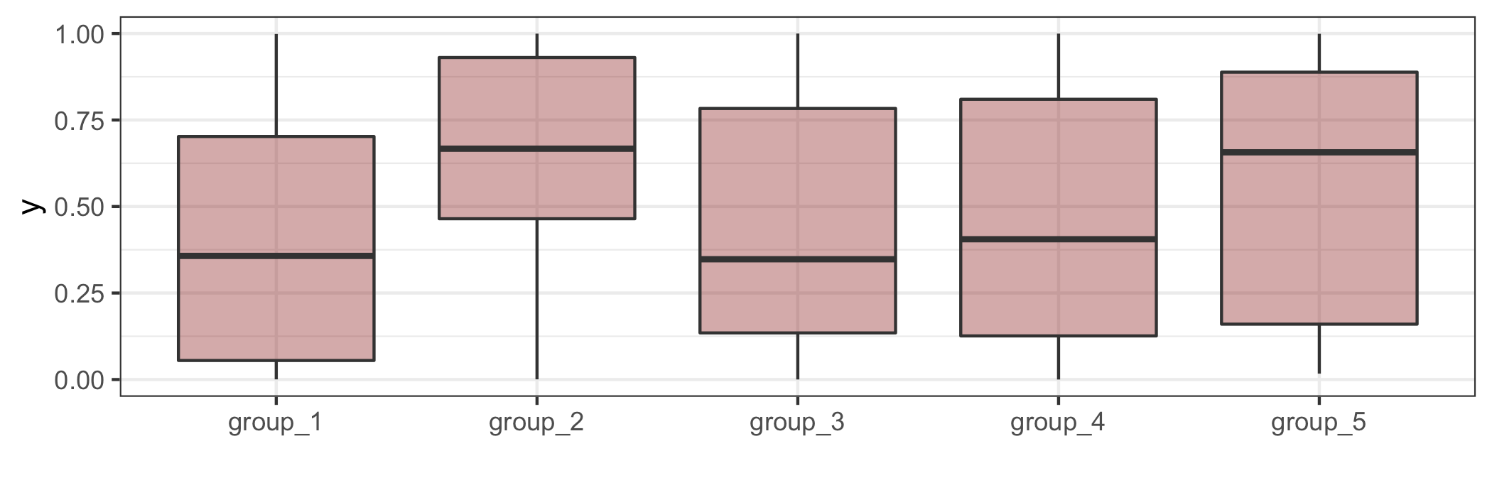 |
| Heatmap | geom_tile( x, y, params ) | 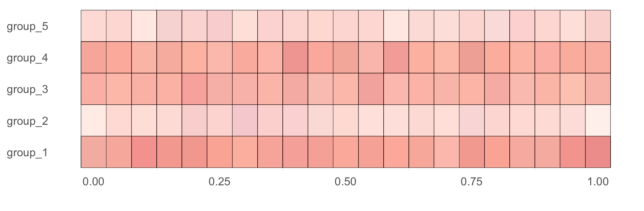 |
where the possible parameters are summarized in the table below:
| Command | Description | Example |
color | Color of a line / point / border | 'red' |
fill | Color of an area | 'red' |
size | Size of a line / point | 4 |
shape | Shape of a point | 4 |
linetype | Shape of a line | 'dashed' |
alpha | Transparency, between 0 and 1 | 0.3 |
Remark: this reference provides an extensive list of possible colors.
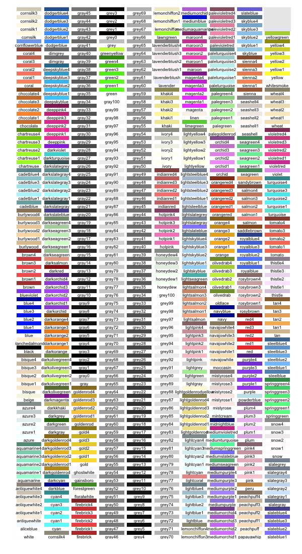
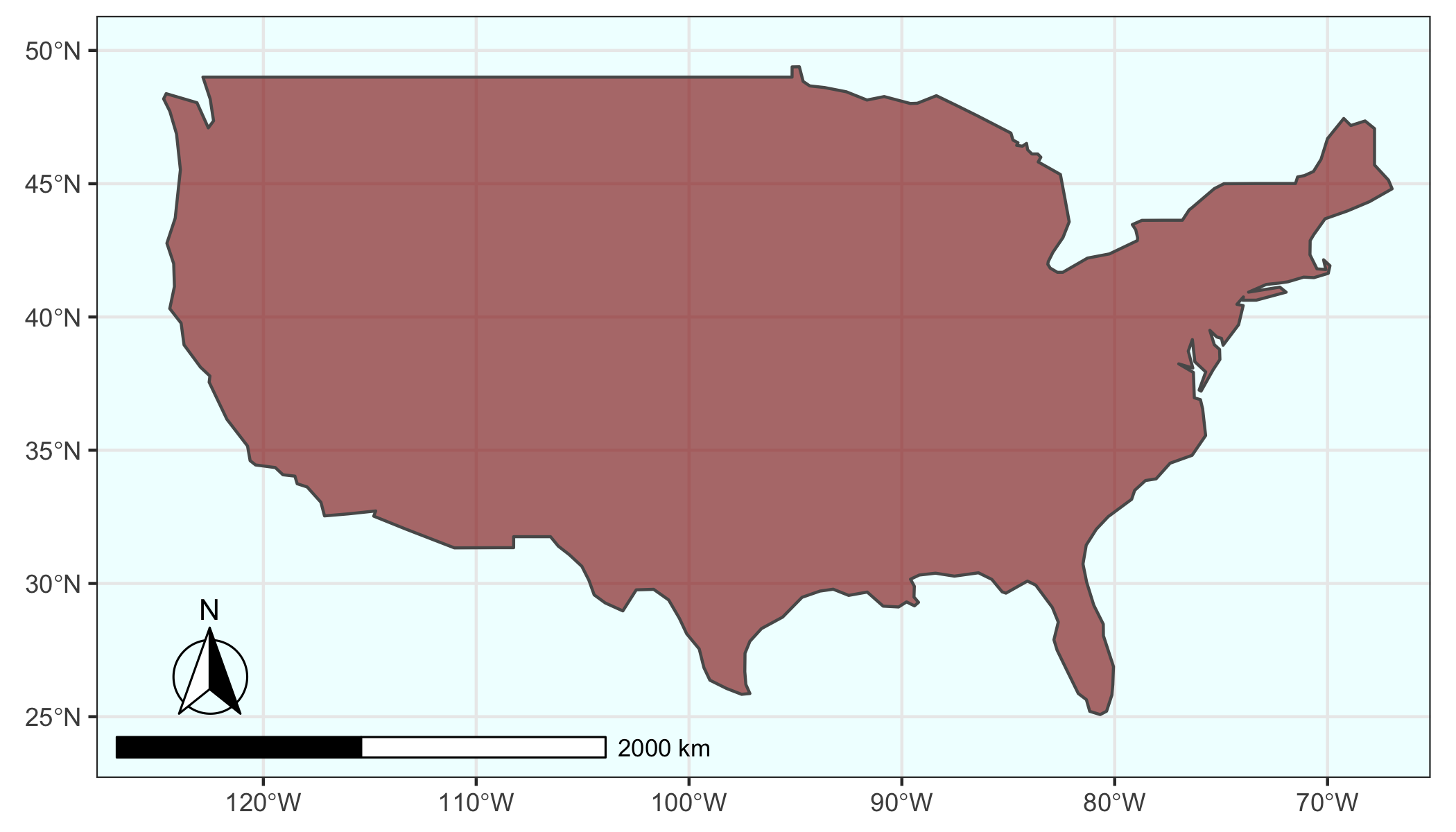
Maps It is possible to plot maps based on geometrical shapes as follows:
The following table summarizes the main commands used to plot maps:
| Category | Action | Command |
| Map | Draw polygon shapes from the geometry column | geom_sf(data) |
| Additional elements | Add and customize geographical directions | annotation_north_arrow(location) |
| Add and customize distance scale | annotation_scale(location) | |
| Range | Customize range of coordinates | coord_sf(xlim, ylim) |
Animations Plotting animations can be made using the gganimate library. The following command gives the general structure of the code:
# Main plot
ggplot() +
  ... +
  transition_states(field, states_length)

# Generate and save animation
animate(plot, duration, fps, width, height, units, res, renderer)
anim_save(filename)
Advanced features
Facets It is possible to represent the data through multiple dimensions with facets using the following commands:
| Type | Command | Illustration |
| Grid (1 or 2D) | facet_grid( row_var ~ column_var ) | 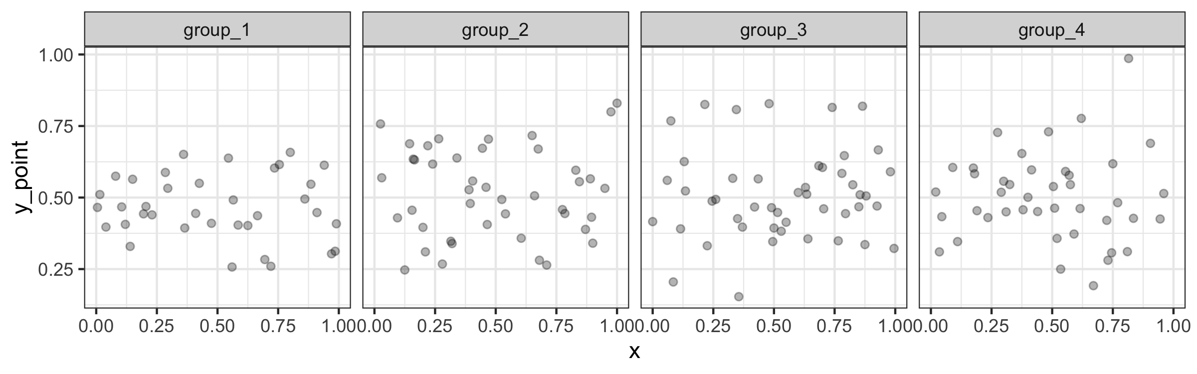 |
| Wrapped | facet_wrap( vars(x1, ..., xn), nrow, ncol ) | 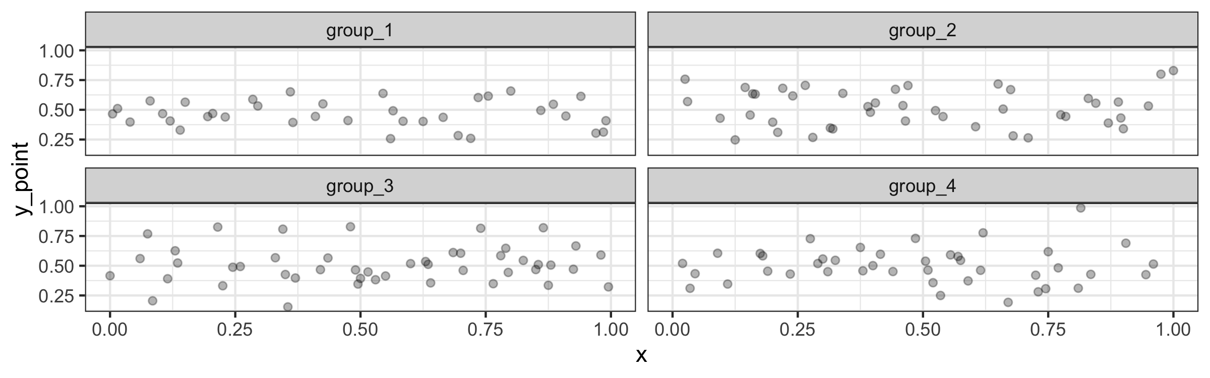 |
Text annotation Plots can have text annotations with the following commands:
| Command | Illustration |
geom_text( x, y, label, hjust, vjust ) | 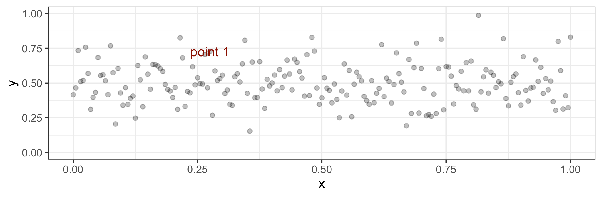 |
geom_label_repel( x, y, label, nudge_x, nudge_y ) | 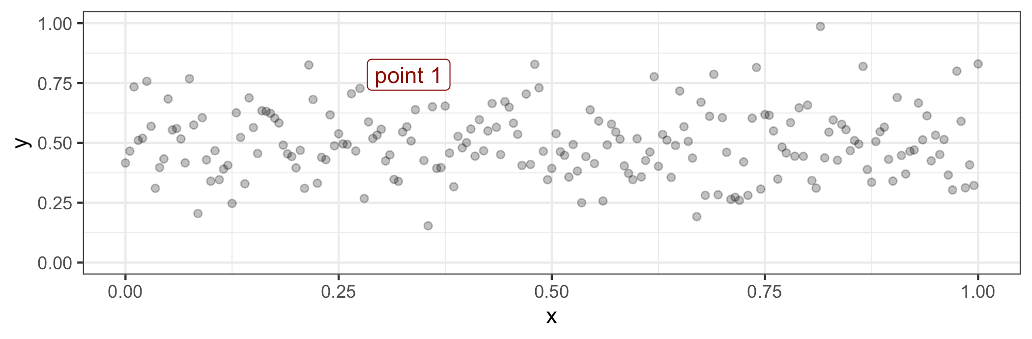 |
Additional elements We can add objects on the plot with the following commands:
| Type | Command | Illustration |
| Line | geom_vline( xintercept, linetype ) | 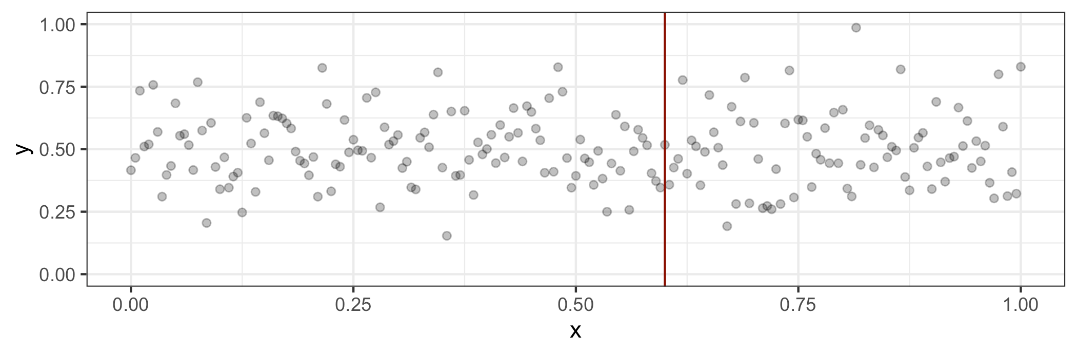 |
geom_hline( yintercept, linetype ) | 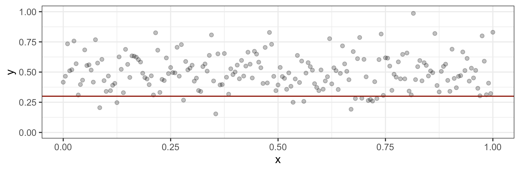 | |
| Curve | geom_curve( x, y, xend, yend ) | 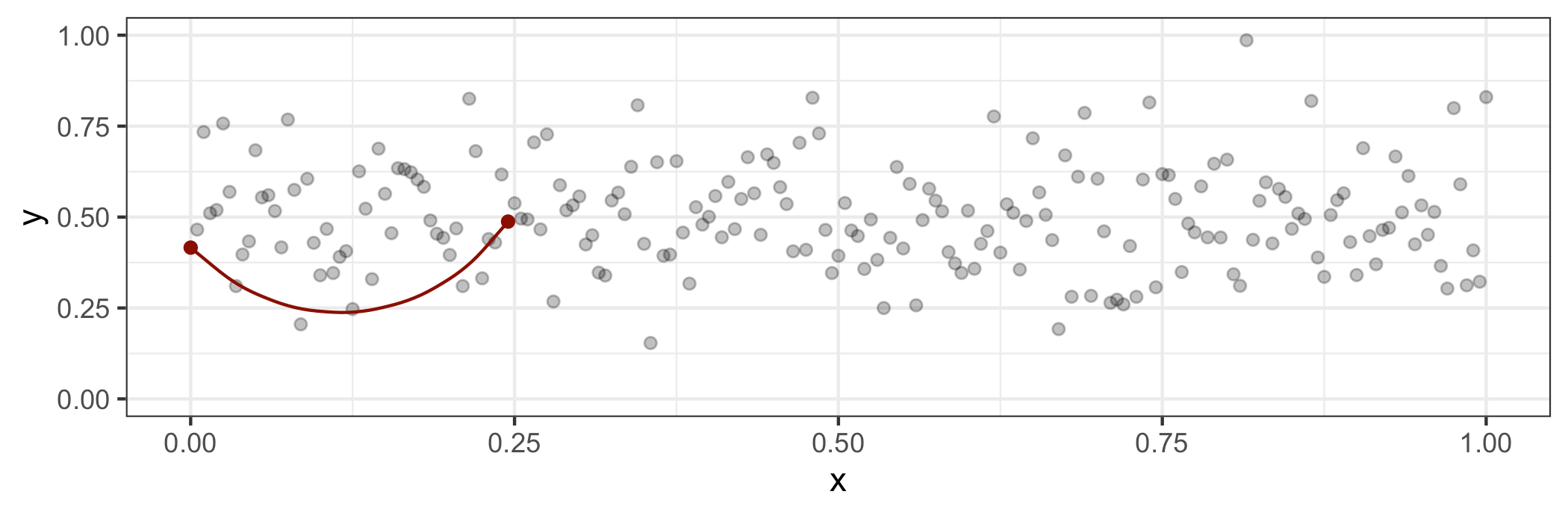 |
| Rectangle | geom_rect( xmin, xmax, ymin, ymax ) | 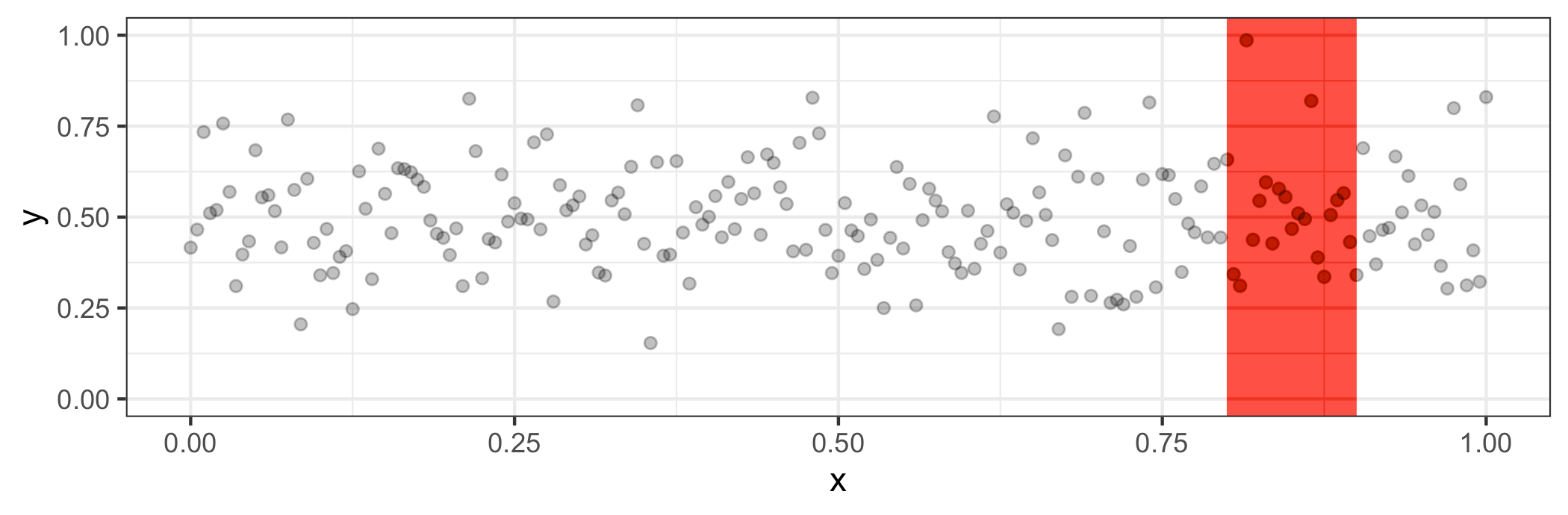 |
Last touch
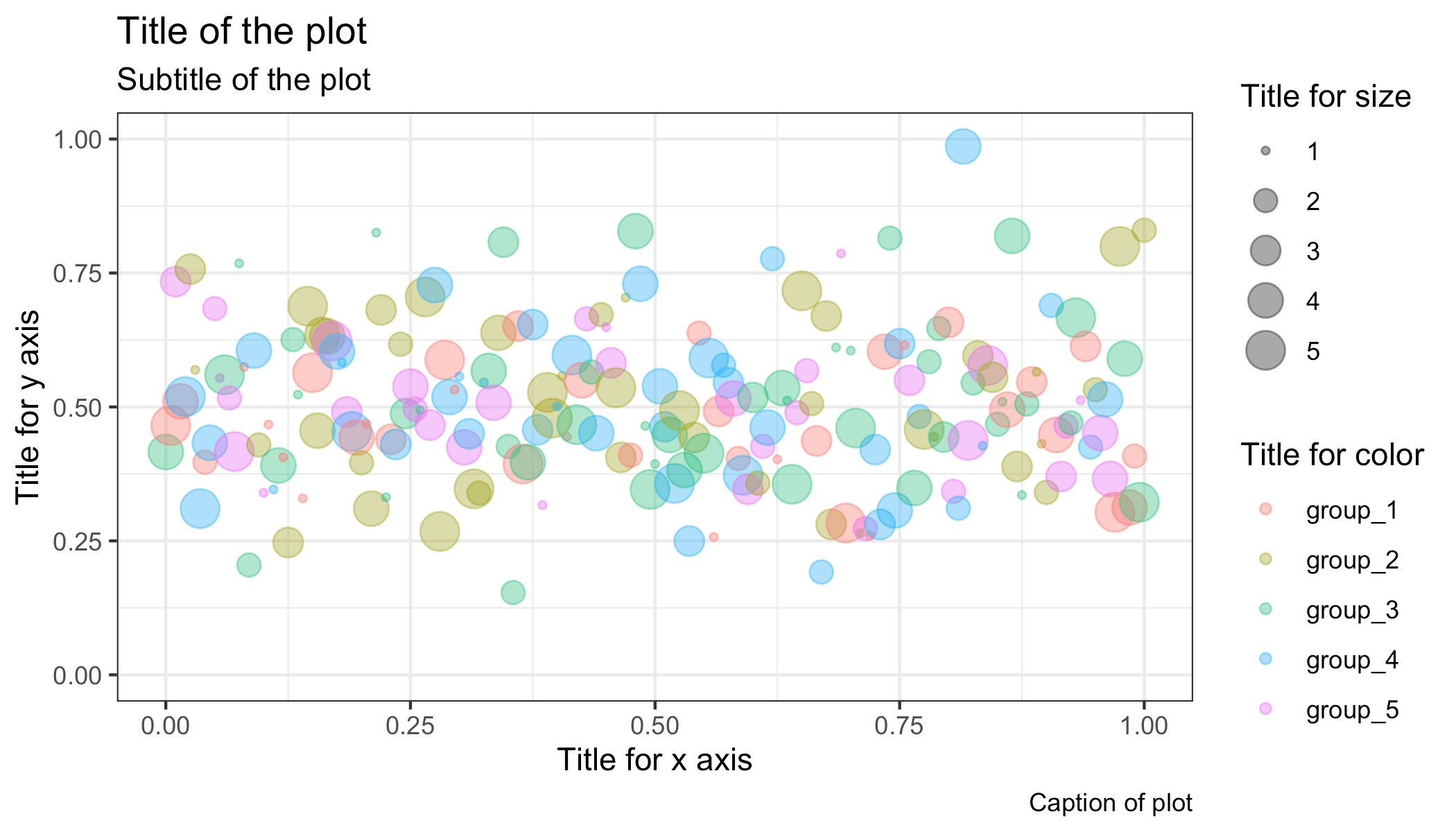
Legend The title of legends can be customized to the plot with the following command:
plot + labs(params)
where the params are summarized below:
| Element | Command |
| Title / subtitle of the plot | title = 'text' / subtitle = 'text' |
| Title of the $x$ / $y$ axis | x = 'text' / y = 'text' |
| Title of the size / color | size = 'text' / color = 'text' |
| Caption of the plot | caption = 'text' |
This results in the following plot:
Plot appearance The appearance of a given plot can be set by adding the following command:
| Type | Command | Illustration |
| Black and white | theme_bw() | 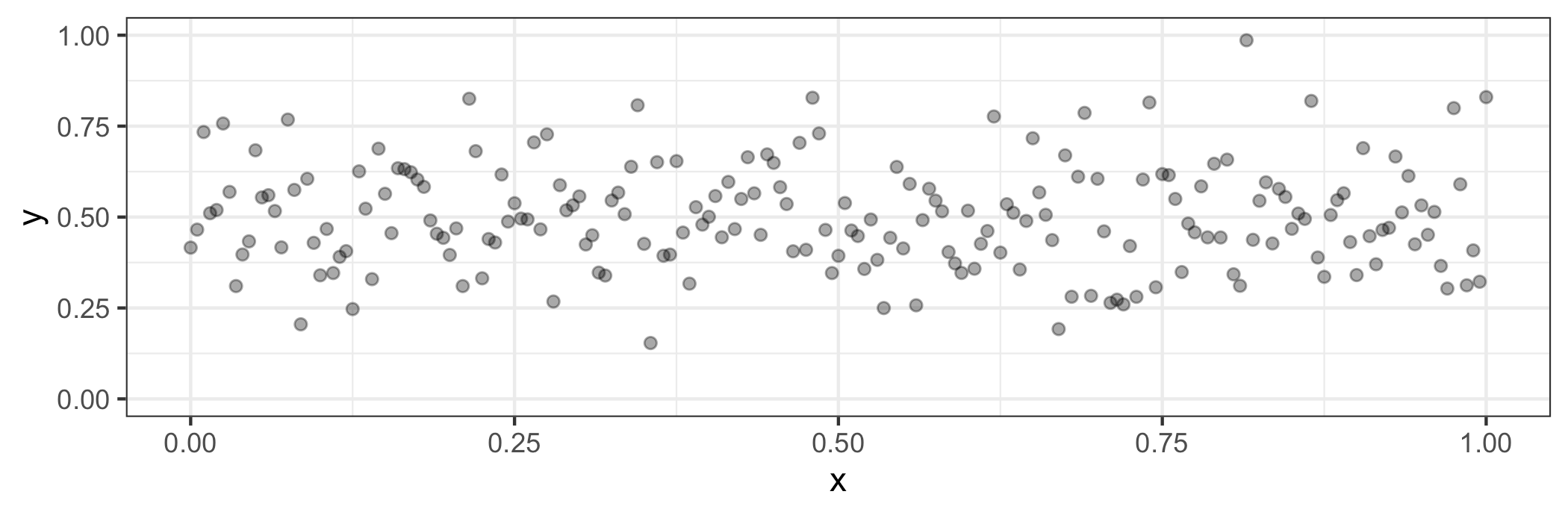 |
| Classic | theme_classic() | 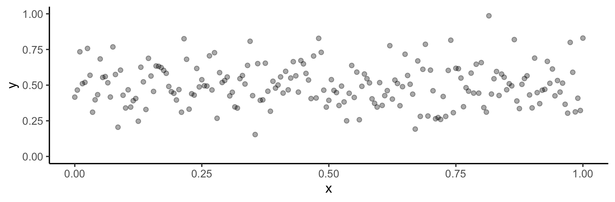 |
| Minimal | theme_minimal() | 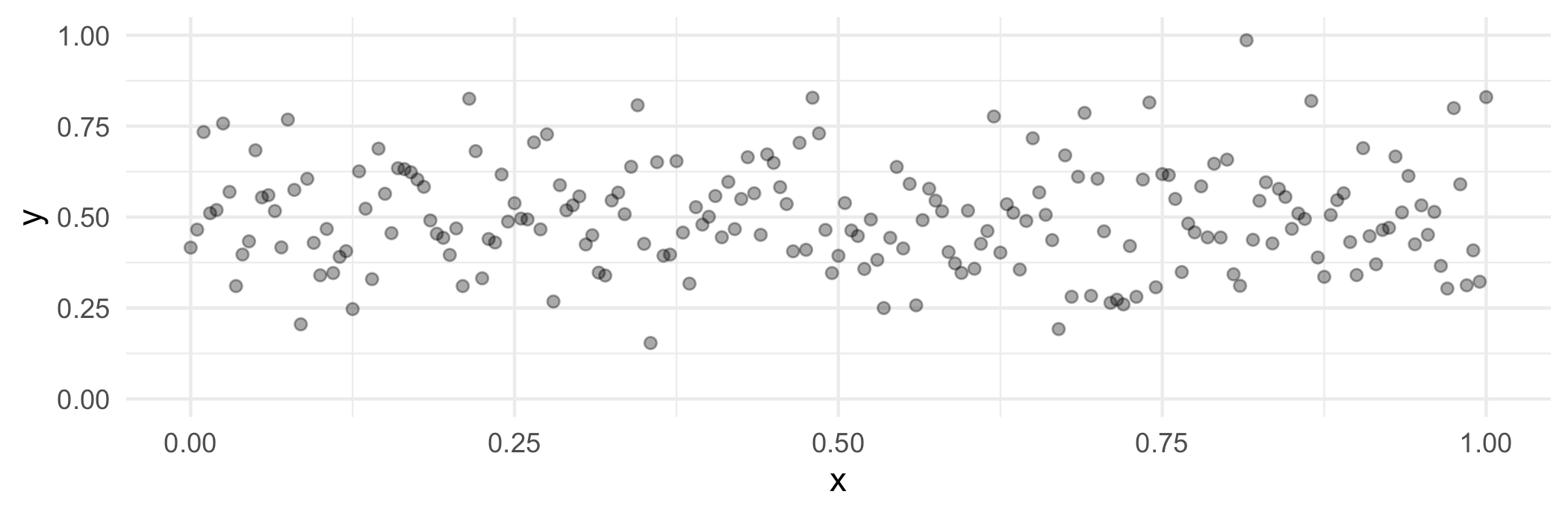 |
| None | theme_void() | 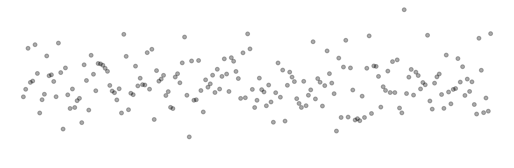 |
In addition, theme() is able to adjust positions/fonts of elements of the legend.
Remark: in order to fix the same appearance parameters for all plots, the theme_set() function can be used.
Scales and axes Scales and axes can be changed with the following commands:
| Category | Action | Command |
| Range | Specify range of $x$ / $y$ axis | xlim(xmin, xmax) |
ylim(ymin, ymax) | ||
| Nature | Display ticks in a customized manner | scale_x_continuous() |
scale_x_discrete() | ||
scale_x_date() | ||
| Magnitude | Transform axes | scale_x_log10() |
scale_x_reverse() | ||
scale_x_sqrt() |
Remark: the scale_x() functions are for the $x$ axis. The same adjustments are available for the $y$ axis with scale_y() functions.
Double axes A plot can have more than one axis with the sec.axis option within a given scale function scale_function(). It is done as follows:
scale_function(sec.axis = sec_axis(~ .))
Saving figure It is possible to save figures with predefined parameters regarding the scale, width and height of the output image with the following command:
ggsave(plot, filename, scale, width, height)