
| Introduction | VRUT and Python? |
| Topic 1 | Building a simple world |
| Topic 2 | Understanding coordinate systems |
| Topic 3 | Creating your own 3D objects |
| Topic 4 | Applying textures |
| Topic 5 | Using lights |
| Topic 6 | Embedding user interaction |
| Topic 7 | Using callbacks for animation |
| Topic 8 | Using sensors (eg. head tracking) |
| Topic 9 | Python tricks for building experiments |
| Topic 10 | Advanced viewpoint control |
| Topic 11 | Advanced texture methods |
| Topic 12 | Controlling hierarchical models |
| Topic 13 | Tips for increasing performance |
To build a complex environment that includes interaction, you must learn how to create scripts. To do this, youll use a language called Python that is simple to use yet very powerful. If youve had any programming experience, youll quickly see that Pythons interpreted style programming is as easy as BASIC. If youve never programmed before, dont worry, this is a great language to start with and youll soon discover how just a half page of python code can generate interesting environment-user interactions.
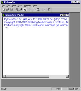
To give you a feel for what VRUT is like, well start with a simple example. First, you must launch the Python interpreter (called Pythonwin on PCs). It will look something like this:
Quick demonstration
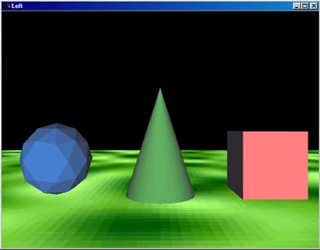
Now, lets fire up VRUT and see a simple demo. To do this, type the
following statement the Python command prompt (the picture below shows
what should appear on your desktop):
>>> import tutorial
Try pressing the "1", "2", or "3" keys on the keyboard and see what happens (keyboard input is only registered with the VRUT graphics window is the active or topmost window). Beside the graphics window, youll see that a text-based window also appears, referred to as the console window. As youll discover, the console window is where youll get feedback about VRUT runtime errors so you should get in the habit of reviewing its contents when things arent working as expected.
NOTE: to run the demo after its first invocation within the same Python session, you must use a different command (remember this because unless you dont this oddity of Python will no doubt come back and haunt you):
>>> reload(tutorial)
Python tutorial
The rest of this tutorial will show you how easy it is to build interactive
environment such as this example. But before you continue with the next
step, its strongly recommended that you spend 45 minutes reading through
the official Python tutorial here. This
is a great tutorial that will quickly teach you all the basics of the Python
language apart from the VRUT 3D graphics. Dont worry if you cant make
it all the way through the tutorial on your first try--just get as far
as you can in 45 minutes and then refer back another day to learn more.
You wont regret investing the time now learning the basics before continuing
with the VRUT tutorial.
OpenGL hardware support
Heres a quick note about hardware acceleration: VRUT should work on
any WIN95/98/NT machine, but unless you have some form of hardware graphics
acceleration, you probably wont be too pleased with the performance. If
the demo you ran above ran but showed really slow or stuttering animations,
then you probably dont have hardware acceleration. If youre in the market
for upgrading, what you need is an OpenGL graphics card (good versions
of these can be easily found for little over $100). The main OpenGL
website has a list of these graphics cards along with reviews.
>>> import vrut
VRUT 2.2
Now, you can enter VRUT commands. After loading the VRUT module, the first command that must precede all others is
>>> vrut.go()
This launches the render and console windows of VRUT (which is also referred to as WINVRUT on PCs) and sets up these windows as the recipient of all subsequent VRUT commands. For instance, you can now issue a command to change the background color by clicking on the Pythonwin window and typing
>>> vrut.clearcolor(0,0,1)
This changes the background color to solid blue. Typing that command before starting the render window with vrut.go() would have had no effect unless the render window is currently running, any commands you send it from the Python interactive window will have no effect whatsoever.
Adding 3D objects
You should think of the render window as an empty world that is waiting
to have some 3D objects loaded into it. Whenever the world is empty, VRUT
will spin a cube with the VRUT logo on it just so you know its alive.
As soon as you tell it to load a 3D object, the splash screen will disappear
and youll see your object instead. Try starting an empty world and then
loading an example object by typing:
>>> vrut.go()
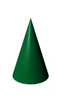
>>> c = vrut.addchild(tut_cone.wrl)
You should now see a cone in view straight ahead. To make things more interesting, add a ground surface:
>>> vrut.addchild(tut_ground.wrl)
Navigating by mouse control
Now its time to try moving around a bit. The easiest way to check
out your handiwork is to navigate with the computers mouse. The builtin
mouse navigation mode is like an automobile. You set the mouse pointer
to the middle of the render screen and then press the LEFT mouse button.
To move forward, ease the pointer upwardthe farther up the faster youll
go. To move backward, ease the pointer downwardagain adjust speed by the
distance you move the pointer from the center of the screen. To steer,
push the pointer to the left or right simultaneous with forward or backward
motion. At first it may be a little difficult to move around but with practice
youll get used to the control interface.
Now lets add a few more obstacles so you can test your steering skills. Add more objects by typing:
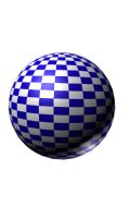
>>> s = vrut.addchild(tut_sphere.wrl)
>>> b = vrut.addchild(tut_box.wrl)
Modifying objects
Easy to slalom between these obstacles you say? What if we make the
objects bigger? Its easy to modify 3D objects once theyve been loaded
into VRUT. One way you can change objects is to scale them up or down.
Try scaling cone to make it larger. To modify an object, you must access
it through its built-in functions. You may have noticed from above that
when the "cone" was added to the world, we assigned it to the variable
"c". By doing this, it allows us to access functions that belong to the
object that act directly upon it. Notice no variable was assigned to the
"ground" object; this means once it is loaded we will never be able to
modify it. If you ever think you might modify an object, assign it to a
variable. Now try scaling the cone:
>>> c.scale(2,1,2)
This made the cone twice as wide but didnt change its height. Note also there there is no "vrut" in this command. The reason for this is that the scale command is a "method" of the VRUT object returned by the addchild command. It is still a vrut command, though. As you see, the scale command requires three parameters--one for each dimension. Numbers less than one will shrink the object and numbers greater than one will expand the object. To the cone to its original size, issue
>>> c.scale(1,1,1)
To start all over, quit VRUT by hitting <ESCAPE> or clicking on the close-box on either VRUT windows. This completely clears all the VRUT commands youve issued even though they will still appear on the Python interpreter window. To start a new world, simply enter vrut.go()and an empty world is created again.
Putting commands in a script
Although its useful for learning, typing in commands over and over
at the Python prompt gets tedious. Luckily, as youve already discovered
in going through the Python tutorial, theres a convenient method for storing
commands as a script and then running them in batch mode. To do this, you
simple store all the commands in a text file, save it with a .py extension,
and then use the import command to execute your saved script. As an example,
well try entering the commands of the simple environment built above into
a Python script.
If youre using Pythonwin, start a new python script window and enter the following lines:
# This is my first python script
import vrut
vrut.go()
c = vrut.addchild(tut_cone.wrl)
s = vrut.addchild(tut_sphere.wrl)
b = vrut.addchild(tut_box.wrl)
c.scale(2,1,2)
Then, save the file as "simpleworld.py" in an appropriate directory thats included in your search path (you may need to ask someone else which directories VRUT/Python uses). Finally, run your script by typing:
>>> import simpleworld
And remember, to run the script after the first successful invocation, you have to type:
>>> reload(simpleworld)
Search paths
You may be wondering where Python and VRUT look for scripts and other
files. The default location is your current working directory. This means
that if you place all your project files in a folder and set Pythonwins
current directory that folder, then all your files should get found without
a hitch. There are two methods to set the current working directory. One
way is to use the standard file dialog box and set it to show your desired
directory. This will then be used when loading scripts from the command
line and by VRUT when loading geometry and textures. Alternatively, you
can use the Python standard library "os" to issue an "os.chdir()" command
that will change to a given directory. This trick is sometimes handy for
embedding within a script if you want to change the working directory on
the fly.
In 3D space, the smallest area that it is possible to occupy is a point. Each point is defined by a unique set of three numbers, called coordinates. An example would be the coordinate (0,0,0), which defines the center point of 3D space, also called the origin point. Each point in virtual space is specified by three coordinates comprising the horizontal, vertical, the depth components.
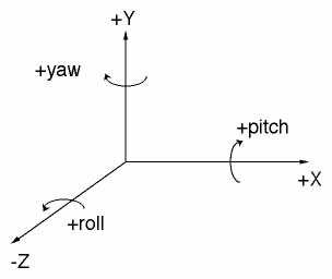
An axis is an imaginary line in space that defines a direction. There are three standard axes in VRUT, which are referred to as the X, Y, and Z axes, as shown in the figure below. As you can see, X is width, Y is height, and Z is depth. Note also the sign of the axes: positive X points to the right, positive Y points up, and positive Z points away or into the screen. These axes are normally fixed relative to the world.
With the mention of meters above, you may be wondering if units are important in virtual environments. They are extremely important. VRUT has many built-in assumptions, and one important assumption is that the linear unit is always meters (this becomes especially important when trying to render perspectively correct stereoscopic imagery). So, when you later build your own 3D models, remember to size and locate them in meters.
Translation and rotations
Lets test out the coordinate system by testing our ability to translate
3D objects along the various axes. Well start by building up a simple
world again with the following commands:
>>> import vrut
VRUT 2.2
>>> vrut.go()
>>> h = vrut.addchild(tut_hedra.wrl)
You probably just see a ground surface and no other objects. Thats because the hedra you loaded (object "t") has a default location at (0, 0, 0) and therefore is right under your nose. To see it, move the viewpoint straight back using the mouse. You should now see a hedra in front of you. Now, try moving the hedra to the right by typing:
>>> h.translate(1, 0, 0)
That moved the object positive 1 meter along the X axis. If it didnt move to the right then that means you didnt move the viewpoint straight back. The translate command uses world axes which means motions occur along axes fixed to the world. If you move the viewpoint so its now looking down the negative Z axis instead, X translations will be completely reversed relative to axes attached to the viewpoint.
Now try moving it negative 1 along the X axis. As you probably guessed, the parametersr for the translate command are (x, y, z). Try moving the object along the Y and Z axes also. By now youve probably noticed that each time you issue the translate command, you replace an previous translations with the new location. If you want to reset the hedra back to its original location, all you have to do is translate it to (0, 0, 0).
What about rotations? Its just as easy to rotate an object as it is to translate an object; you use the rotate command. The parameters for the rotate command are (x, y, z, angle). The first three parametersx, y, and zform a vector that define the axis about which the rotation will take place. The fourth parameter, angle, is the amount in degrees to rotate. Try rotating the hedra by 45 deg about the vertical axis:
>>> h.rotate(0, 1, 0, 45)
Next, try rotating along the X and Z axes again by 45 deg and see what results. Look at the axes figure above to see the direction of positive angles about the principal axes as indicated by the arrows.
If you use rotations much in the environments you build, youll no doubt discover a complication with rotations that doesnt occur with translations. This complication is that the axis of rotation must pass through a specific point in the virtual space. In the example above, the hedra was built to rest on the ground surface at the origin. Its dimensions are 1x1x1 m, so that means the location of its center is (0, 0.5, 0). Did you notice that when you rotated about both the X and Z axis, the object did not rotate about its center and yet it did for the Y axis? Thats because all VRUT objects have a default rotation centerpoint set to the origin (0, 0, 0). If you want this object to rotate about its center regardless of axis, you must override the default centerpoint by typing:
h.center(0, 0.5, 0)
Now, try rotating about the X and Z axes and see how the effects are
different now. You may wonder how you know where the center of the object
is. Right now, the only way is to keep track when you build the object
in your modeling program. A good habit so you dont have to keep track
it to always center your objects about the origin; itll later simply rotations.
VRUT can directly import 3D models that are stored in the latest version of VRML (Virtual Reailty Markup Language 2.0 / 97); earlier versions of VRML are not compatible and will not load at all. For those new to VRML, it is, amongst other things, a format for specifying 3D objects that has become a popular standard for exchanging 3D data. To find out more about VRML and where its going, see www.web3d.org (formerly www.vrml.org).
VRML modelers
The only practical way to build VRML models is to use a commercial
3D modeling package that exports VRML output files. There are many such
products available, including 3D Studio, CosmoWorlds, and AC3D (this package
is shareware and can easily be downloaded to quickly get started though
its not recommended for serious model building). Both 3D Studio and CosmoWorld
are powerful modelers that require a serious investment of time to learn
how to use. This tutorial doesnt provide guidance to learning these modelers
and its recommended that you find dedicated tutorials written by the pros
(for your specific modeler).
To help you get started, VRUT comes with a bunch of VRML files already loaded that you can start piecing to together to build simple environments. Heres a list of the files that should be loaded on your system:
<list VRML files>
A useful exercise is to open a VRML file in a text editor and view its contents. If you choose a simple enough 3D object, youll probably be able to look through the contents of the file and understand most of its contents. This is sometimes useful to figure out why certain things youre building may or may not be working. It may also come in handy sometime if you need to make a simple change to a model file and you dont have access to your fancy modeling package (eg., changing the name of the texture or color of an object is very straightforward). Try looking at tut_cone.wrl and tut_box.wrl and seeing what the differences are between these two VRML files.
tut_cone.wrl
tut_box.wrl
#VRML V2.0 utf8
# Produced by 3D Studio MAX
VRML 2.0 exporter, Version 2, Beta 0
DEF Box01-ROOT Transform {
translation
3 0.06863 -8
children
[
Transform {
translation 0 0.85 0
children [
Shape {
appearance Appearance {
material Material {
diffuseColor 0.8784 0.3373 0.3373
}
}
geometry Box { size 1.7 1.7 1.7 }
}
] }
]
}
Unsupported VRML features
Unfortunately, the VRML loader that is currently used to support VRUTs
needs is limited and does not support many of the extensive features of
VRML97. The features that are not supported are the following (though VRUT
provides methods for doing many of these):
| level of detail | touch sensors |
| proximity sensors | scripting |
| viewpoints | navigation info |
| switches | protos |
| animated textures | anchors |
| background |

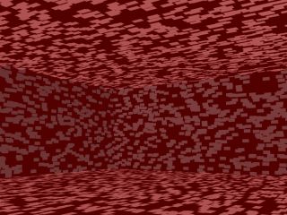
This scene contains 7,000 bricks. Each brick has 4 vertices (corners), and each corner has 3 coordinates (X, Y, Z). This scene contains 84,000 coordinates that must get send through the geometry pipeline each time a graphics frame is rendered.
Before special texture mapping hardware became available, there was no other choice than to use the method above. But thats history, and now specialized texture mapping hardware is available everywhere. What texture mapping allows you to do is build a single polygon and to then wallpaper it with a 2D image. We can now replace an entire wall from the example above and map it with the following image to get this result.

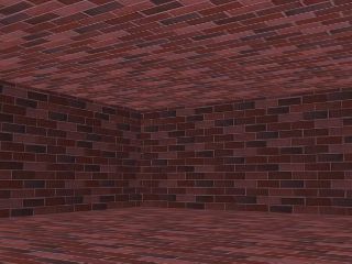
Now, the scene contains just 6 polygons resulting in a total of 72 coordinates to flow through the graphics pipe. Youll soon discover that the fewer polygons you throw at the graphics pipe the faster youre virtual environments will run in terms of framerates. By using textures, we get the added scene complexity literally for free in terms of rendering performance thanks to the dedicated hardware.
Tiling
Another powerful features of texture mapping is that you can play with
the way in which a texture gets mapped onto the polygons. In the example
above, the brick image was mapped one-to-one onto each polygon of the room.
If we want to make the bricks bigger, all that has to be done is to "tile"
the brick image onto the polygon many-to-one. For instance, heres what
the scene would look like by tiling the bricks one-half in each direction.
You can also do the opposite and only use a portion of an image to zoom in to a specific portion per polygon. Actually, that is precisely the technique used to "wrap" a 2D image around a 3D object. Below is shown the same brick image wrapped once around a cylinder. Any 3D modeler worth using will do texture tiling and texture wrapping automatically for you.
A handy feature of some textures is that they are seamlessly tile-able. Here are two texture that may look similar at first glance but when one shows obvious tiling boundaries while the other does not.
Supported formats
Textures themselves are nothing fancy. In fact, textures are nothing
more than bitmap images that are stored in standard formats. You can use
a number of methods to capture textures, including digital cameras, scanners,
and paint programs. VRUT supports many standard image formats so its easy
to use images you may already have access to. VRUT also comes with a large
collection of textures that you can use when building virtual environments.
To see these, look in the VRUT installation directory under /texture. If
you want to develop your own textures for using with VRUT, there are a
few simple rules that you should bear in mind.
Texture files must meet the following requirements:
The other two choices, spot and point light sources can be used to create special effects. A spot light casts a cone of illumination that can be adjusted to have either a sharp or soft edge around the circular illumination area. A point light source is much like a candle, it casts light in all direction equally but the intensity falls off with distance. If you want to use either spot or point lights to create special effects, keep in mind that your geometry must be tesselated in order to take full advantage of these partaicular lighting effects Tesselation is the process of sub-dividing an object into smaller subcomponents. For example, to properly use a spotlight on a flat square, the square would have to be composed of many sub-squares so that OpenGL can differentially illumate and interpolate across the individual vertices. You can easily experiment with these effects by building an object in your modeler and changing the level of tesselation and look at how lighting effects are affected.
Enabling lighting
By default, lighting is disabled with respect to texture mapping, meaning
any surfaces with texture will have no shading effects. Also by default,
there is a universal directional light pointing down the positive Z axis
that will produce shading effects on non-texture mapped geometries. This
light exists so that you can easily view models without worrying about
lighting. To disable both of these default modes, you must issue the following
command without any parameters:
>>> vrut.override()
Locking light visibility
When you add lights using VRML files, you should keep in mind several
aspects of how VRUTs scene graph works. First, lights will affect the
child object in which they are stored and all subsequent objects below
(after) it, but a light will not affect object above (before) it. So, if
you want a light to apply to all your geometry and you are loading your
geometry from several files, load the geometry with the lights first. Second,
a light that is loaded along with geometry will be active (turned on) only
as long as the associated geometry is within the field-of-view (view frustum);
once all the geometry for that object moves out of view either due to a
translation or viewpoint rotation, the light is turned off. This is part
of OpenGL Optimizer that automatically culls geometry objects that are
not in view from the render cycle. It has the unfortunate effect of turning
off lights you might otherwise wish left on. To get around this problem,
you lock down all lights within a geometry object so that they can never
be turned off. To do this on an object by object basis, you the objects
"appearance()" method and pass it the parameter "vrut.LOCKLIGHTS".
<object>.appearance(vrut.LOCKLIGHTS)
Lighting works by blending three different colors: the light source, the texture map if present, and the underlying material color of the object. If you simply want shaded but otherwise un-colored texture mapping, you should assign all material and light colors to white (in your VRML editor).
The current version of VRUT does not provide any shadow effects.
Callbacks
Whenever VRUT detects that a form of user input has occurred, it generates
what is known as an "event". In order to respond to an event, you as the
programmer can write a Python function that gets called whenever that particular
event occurs. For example, you might want to "trap" keyboard events in
your virtual environment, so you would write a function to handle key presses
and this function will automatically get called by VRUT whenever the user
presses a key on the keyboard. A function that gets called whenever an
event occurs is known as a "callback" function. If youve never written
event style programs before, youll find this concept strange at first
because youre probably not accustomed to writing functions that are never
explicitly called somewhere else in your program. You must get used to
the fact that VRUTs event manager will call your function for you whenever
necessary.
Keypresses
Although callback functions can be named and contrain whatever you
desire, they must be written to accept a pre-defined argument list that
depends on the type of function. A keyboard event callback function must
be written to accept a character-type argument; this will then contain
the key pressed by the user. Heres an example of a what a keyboard callback
function might look like:
# This function is triggered whenever a keyboard
button
# is pressed and gets passed the key that was
pressed
# into the argument whichKey.
def mykeyboard(whichKey):
print The following key was pressed: , whichKey
As youll see, once the code above is setup to be called by VRUT whenever a keyboard event occurs, VRUT will print the sentence "The following key was pressed: --" showing the key actually pressed.
To add to the complexity of handling events, there is an additional command you must include besides writing the code for the callback function. You must register the callback function so that VRUT is aware that it exists and knows to call it whenever the appropriate type of event occurs. This is simple, and for trapping keyboard events using the function above the statement looks like:
vrut.callback(vrut.KEYBOARD_EVENT, mykeyboard)
Thats all there is to it. Lets try putting everything together and testing out your own callback. Heres the program weve built above all put together. Try typing this into a blank Pythonwin script document, saving it, and then running it.
# This is my first program using callbacks
import vrut
vrut.go()
color = 0
# This function is triggered whenever a keyboard
button
# is pressed and gets passed the key that was
pressed
# into the argument whichKey.
def mykeyboard(whichKey):
global color
color = color ^ 1
vrut.clearcolor(color, color,
color)
print The following key was
pressed: , whichKey
vrut.callback(vrut.KEYBOARD_EVENT, mykeyboard)
When you run this program, you should simply see the VRUT splash screen with the spinning cube running. Try hitting a key on the keyboard. You see two things happen: 1) everytime you press a key the background color changes between black and white, and 2) the console screen prints out a message telling you which key was pressed. Though this is just a simple example, you can image how you can add some Python code so that it responds in ways that depend on which key was pressed (i.e., adding an "IF" statement).
Mouse & hotspot events
In addition to trapping keyboard events, you can also instruct VRUT
to signal you whenever the user presses a button on the mouse or even just
moves the mouse. Yet another handy type of event you can set up is one
that triggers when the users viewpoint enters a region of the virtual
environment that you specify. This latter type of event is called a hotspot
event.
Here are two Python programs that show you how to use MOUSE_EVENTS and HOTSPOT_EVENTS. Try looking at these programs, seeing what they do, and running them.
<tutorial_hotspot.py - Still under construction>
<tutorial_mouse.py - Still under construction>
The trick to regaining control of the execution cycle is to use timer events. VRUT allows you to start what are called "expiration timers", timers that will trigger a TIMER_EVENT when their time interval expires. You can then use that timer event to coerce VRUT into running your registered timer callback function, and in that function you can do whatever you wish to animate objects (or yet other things). For example, if you want to translate an object once every tenth of a second, then you set up a timer to go off every 0.1 sec. Each time it goes off, you can incrementally translate the target object. To achieve really smooth animations, youll want to set up your timers to expire once every frame. Depending on your hardware, your maximum frame rates are going to be somewhere around 60 Hz. To play it safe, you can set a very short expiration time like 0.001 sec which will ensure that you always have a timer expiring every frame. And dont worry, they wont stack up and waste performance because once a timer expires, you must trigger it again. Youll see this in the example below.
Rotation
This example shows how to render an animation of a hedra spinning about
the vertical axis. There are several important things you should notice
in this program. First, notice how every time we run the timer callback
function ("mytimer"), we set up a new timer so that it will keep expiring
every frame with the vrut.starttimer() command. Second, we have to issue
one vrut.startimer() command outside the callback function to get the whole
thing going for the first time; after that it fuels itself. Third, to render
continuous animations you have to learn how to use the Python "global"
statement so that you can keep track of previous angles and positions.
In this example, removing the "global" statement would cause Python to
forget that the variable "angle" has been incremented each frame.
# This is my first animation
import vrut
vrut.go()
UPDATE_RATE = 0.001
SPEED = 1.5
angle = 0
g = vrut.addchild(tut_ground.wrl)
h = vrut.addchild(tut_hedra.wrl)
def mytimer(timerNum):
global angle
angle = angle + SPEED
h.rotate(0, 1, 0, angle)
vrut.starttimer(1, UPDATE_RATE)
vrut.callback(vrut.TIMER_EVENT, mytimer)
vrut.starttimer(1, 0.5)
Try typing in this program and running it. Remember to step the viewpoint back a little to see the hedra (since its load at the origin). Once youve got this program working fine, try changing some of the parameters and see how they affect your animation. Change SPEED and see what happens? Can you figure out what units SPEED is in? Try changing UPDATE_RATE and see how slow you can make it before you notice any difference.
Translation
Now its time to add a little bounce to the animation. Lets add a
little translation to the animation. Try replacing the timer callback function
with the whats below. Youll also have to add an "import math" to the
top and a new variable named "height" somewhere in the body of the program
(this loads in special math functions so you can access them as youll
see below).
import math
height = 0
def mytimer(timerNum):
global angle
global height
angle = angle + SPEED
height = height + math.sin(angle
/ 20)
height = math.fabs(height)
h.rotate(0, 1, 0, angle)
h.translate(0, height, 0)
vrut.starttimer(1, UPDATE_RATE)
You now know all the basic building blocks for creating complex animations.
By combining rotations and translations, you can get an object to do anything
you want.
To use a tracker with VRUT, the hardware must be properly installed and its own software plug-in must be available. To find out what sensor plug-ins are available on your system, start VRUT and enter vrut.versions(). Look in the section labeled "Sensors" to see what plug-ins are available. Keep in mind, though, that just because a plug-in is available doesnt guarantee that the actual hardware is available. Look through the list and see if you can find the plug-in for the piece of hardware you want to use.
Once youve determined which sensor you want to use, connecting to it is easy. To do this, simply have VRUT running, and then use the vrut.addsensor() command. You pass it the name of the sensor you want to connect to, for example:
>>> s = vrut.addsensor(intersense)
This will cause the computer to open a connection to an "Intersense" head tracking device if its available. If the connection is successful, the variable "s" will be given a value ("s" is actually a VRUT object and remember just as adding object to a world, if you dont assign it to a variable you wont be able to modify them later). If the connection fails, a message will appear and "s" will not be defined.
Quick head tracking
Once youve found a sensor that works, the easiest way to attach it
to the viewpoint so that you can add head tracking to your virtual environment
is to issue the vrut.tracker() command. This command will grab the first
sensor that has been added and connected, and attach it to the viewpoint
using default parameters. This should work for any standard head tracking
device. Try this and see what kind of results you get:
>>> vrut.tracker()
The most common thing youll not like about the default parameters is that the viewpoint may not start pointing in the direction you like. To correct this, you use can reset the tracking device. When resetting, you simply face the sensor in the direction you want to be aligned with the +Z axis in the virtual environment and issue the following command:
>>> s.reset()
This will reset the internal values so that your virtual viewpoint now points due North (+Z). If youre using a sensor that also provides location information about the observer, then likely the reset() command will also center the virtual viewpoint at the origin.
Suppose you want to use the tracking device to move an object instead of the viewpoint. There are two step to accomplish this. First, you use the same method above to connect to the desired tracker. Then, instead of issuing a vrut.tracker() command, you issue the sensor() method command of the geometry object you want it attached to. Heres a program snippet illustrating this process:
box = vrut.addchild(tut_box.wrl)
trk = vrut.addsensor(intersense)
box.sensor(trk)
The object "box" is now under control of the sensor. If the sensor provides orientation data, then the objects orientation will change in real-time to reflect to position of the sensor. If the sensor provides translation information, then objects position will be servoed to the sensor. You can still use the rotate() and translate() method of the geometry object to impose additional transformations that will be superimposed upon the transformation formed from the sensor data.
To remove the sensor from the object, just issue the same command without an argument:
box.sensor()
Accessing sensor data
A final trick you should know is how to access the data from a sensor.
You might want to do this for several reasons, including saving the data
for analysis and filtering the data before using it to transform either
the viewpoint or an object. To access the sensor data, you use the sensors
get() command which will return an array containing the type of data you
requested. The following two forms of the command will return position
and orientation data, respectively:
trk = vrut.addsensor(intersense)
myData = trk.get(vrut.POSITION)
myData = trk.get(vrut.ORIENTATION)
For more information about sensors, read this.
Reading a stimulus file
Well start with an example that reads in a stimulus file that is organized
as tab-delimited columns. Heres an example of what the file might look
like:
1 A
3.5
2 B
2.5
3 C
1.5
4 B
1.5
5 C
2.5
6 A
3.5
With this example, each column will get read into its own array. For the code example below, the name of these three column variables, from left to right, will be trialNum, type, amount. To get Python to read in these columns, you must first open the file in read-only mode. Opening a file returns a Python object that has methods. One of these methods is readlines() which will load and return the entire file. Once the file has been loaded into a local variable, it is straightforward to increment through it line by line to break apart the different parts. The example below illustrates how to do this:
import stringSaving subject data
file = open('stimulus.txt', 'r')trialNum = []
type = []
amount = []all = file.readlines()
for line in all:
s = str.split(line)
trialNum.append(string.atoi(s[0]))
type.append(s[1])
amount.append(string.atof(s[2]))file.close()
file = open('response.dat', 'a')In the example above, the three passed function arguments are assumed to be an int, string, and float, respectively. The function builds an output string by converting any non-string types into a string by using the built-in Python command string(). A handy trick to use when building your output data is to put a TAB character between each item so that the data can then be easily read into a spreadsheet or data analysis program. To specify a tab character in Python, you use a backslash plus the letter t as in \t. Also, if you want each call to SaveData() to begin a new line in the output file, you must force a carriage-return by adding a \n at the end of each line.def SaveData(trialNum, type, response):
out = string(trialNum) + '\t' + type + '\t' + string(response) + '\n'
file.write(out)
file.flush()
Randomizing conditions
If you dont want to bother reading in a stimulus file for your experiment
and you can get away with randomizing your conditions on the fly, then
the example below shows you how to easily setup a random selection without
replacement procedure. This example sets up a hypothetical experiment with
two factors, A & B, having 2 and 3 levels, respectively. A parameter
called "reps" controls the number of repetitions of each trial. To build
up all the stimulus pairs, the script below uses a nested "for"-loop to
build the factorial design by appending each factor pair into a new variable
called "stimulusSet". A standard Python library, "whrandom", is used below
to randomly pick from the stimulus list by using the "choice" command.
After each pick, that item gets removed from the "stimulusSet" list so
that it can never get chosen again. Heres the skeleton code illustrating
this method:
# My first stimulus generator
import whrandomfactorA = ['A', 'B']
factorB = [0.1, 0.2, 0.3]
reps = 5# initialize an empty set so it can be appended to
stimulusSet = []for a in factorA:
for b in factorB:
# append a & b as a trial unit: (a, b)
stimulusSet.append((a, b))# use the * operator to copy set reps times
stimulusSet = stimulusSet * repswhile len(stimulusSet) > 0:
# randomly pick a trial unit from set
trial = whrandom.choice(stimulusSet)
# remove so we dont pick it again
stimulusSet.remove(trial)
print trial, a:, trial[0], b:, trial[1]
Other resources:
Finally, look in the "Resource" pages for sample code of actual experiments
that have been written in VRUT/Python to get an idea how to implement various
other techniques.
Offsets
While its possible to reset a sensor so that the orientation point
due North and position is located at the origin, there are often cases
where you need to add an offset to the viewpoint parameters. For instance,
you might want to push the viewpoint down vertically in a one-time move
to simulate a dogs-eye view. Alternatively, you might want to slowly spin
the viewpoint around the vertical axis so that the user experiences self-motion.
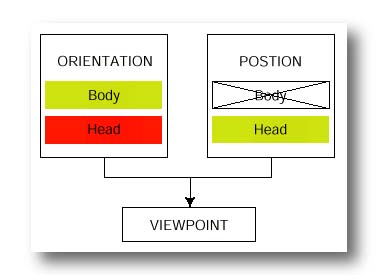
You can manually translate and rotate the viewpoint. To understand how to do this, you need to understand a slight complication. Internally, VRUT maintains two transformations that each contribute to the final viewpoint. These two states are the for the simulated head and body. The reason for representing both of these is to allow you to simulate a user with a body and then to allow the user to move the simulated viewpoint relative to the simulated body. In the current version of VRUT, only rotations use the body transform. If you want to change the orientation of the viewpoint, you modify the body orientation. Head transformations are handled automatically when you turn on automatic head-tracker and get superimposed upon any body orientation transformation that you may have applied. If you want to change the position of the viewpoint, you instead directly change the head position. The diagram below shows values that the user can modify (yellow), values that the system modifies (red), and values that are currently not supported (crossed-out).
>>> vrut.translate(vrut.HEAD_POS, 0, -1, 0)
>>> vrut.rotate(vrut.BODY_ORI, 0, 10, 0)
Each time these command are issued, the viewpoint would move down another 1 m and pitch down another 10 deg. If you want to reset either the head position or the body orientation to the default values, issue either of the two following commands as appropriate:
>>> vrut.reset(vrut.HEAD_POS)
>>> vrut.reset(vrut.BODY_ORI)
Clamps
Opposite to changing the viewpoint is keeping it from changing. There
are situations in which you may want to clamp and prevent from changing
either the head position, head orientation, or body orientation. To do
this, you can use the vrut.clamp() command.
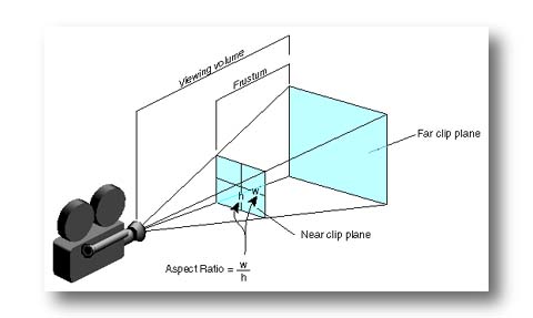
Perspective Transformations
The perspective transformation is used to convert from world space
into device space. This is the stage where 3D data gets mapped onto the
2D screen, and it is critical that the perspective transformation be exactly
correct if you're interested in creating an image that's equivalent with
the way objects in the real world would look.
When VRUT begins, a default perspective transformation is used. In the console mode (the small window typically used for development, or what you get when you just type vrut.go() ), the vertical field-of-view (FOV) defaults to 65 deg. This is a very wide FOV to facilitate development, but beware that the perspective image is only correct for a viewing distance of about 10 cm from the typical monitor! Likewise, in the full-screen modes, the proper viewing distance is still only about 20 cm in order to cast perspectively correct images on your retina. The HMD modes default to what should be close to the correct values for the KEO HMD.
To change the default perspective transformation, you must use the vrut.setfov() command. How to setup correct perspective transformations for both the monocular and stereoscopic are discussed below. To learn how to properly setup a display for either monocular or stereoscopic viewing, follow this link.
![]()
![]()
Transparency is also handy for building shapes that would be virtually impossible to model in 3D, such as natural objects. For instance, rendering a realistic tree can be done using transparency. To do so, you take a photo of a tree and make everything but the leaves, branches, and trunk transparent. What youre left with is a cookie-cutter treeits flat for sure but much simpler to build and faster to render than a complex 3D model of the same thing.
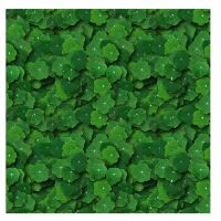
Heres how to add transparency. First, you need a good image manipulation program, such as Adobe Photoshop, that allows you to add whats called an "alpha" layer. An alpha layer is a standard method of specifying visibility or masked regions of an image. If youre using Photoshop, what youll need to do is load an image, go to the "channels" window and add a forth channel (the first 3 should already be for "red", "green", and "blue" components of the image). Photoshops default is for the fourth channel to be used as an alpha layer. Next, you need to select the alpha layer and draw your mask here. For on/off masking, you simply paint anywhere you want to be visible pure white and anywhere you want invisible pure black. The figure below shows a solid green texture that has a large letter "T" made invisible in Photoshop (notice that Photoshop uses a default masking color of red to show you what will become invisible by your rendering software).
![]()
Save the image in a format that retains the alpha layer. The only formats that do this and that VRUT supports are the following: TIF, PNG, and RGBA. When saving in Photoshop, be sure the "Exclude alpha information" checkbox is turned off.
Finally, the default rendering mode is to ignore transparency information. If you want to render transparency, you must change the target objects appearance by issuing the following:
<object>.appearance(vrut.TRANSPARENCY)
Also by default, any region of your texture that has a dark (black) alpha value will render as transparent and any region that has light (white) alpha value will render as opaque. If you want to shift the point along the black/white continuum that mark the threshold between transparent and opaque, use the "alpha()" command to change the threshold point and send it a parameter ranging between 0 and 1. To make only pure white opaque, set the threshold high:
<object>.alpha(1.0)
Alternatively, you blend in tranparency smootly so that the amount of transparency corresponds to the gray-level value of the alpha channel. To do this, you simply turn off the alpha value thresholding by sending no argument to the "alpha" command:
<object>.alpha()
Beware, this method of transparency activates the internal Z-buffer (for handling occlusions) and suddenly the order in which you render multiple transparent objects matters. More specifically, the object that appears first in the scene graph (loaded first) must be located furthest from the viewpoint in order to allow nearer objects to be properly transparent.
**If you aren't seeing an transparency effects, try issuing a vrut.override() command.
Animated textures
Believe it or not, you can watch TV in your virtual environment. Almost,
that is. You can take a sequence of images (e.g., from a Quicktime video)
and use them to play a movie in your virtual environment. The more memory
your rending computer has, the longer the movie can be but dont expect
to show any flicks lasting more than tens of seconds without getting into
trouble. If you have access to any video editing software, such as Adobe
Premiere, its easy to export a video sequence as a series of still and
chose the dimensions of the output images. One caveat about memory usage:
when the images are loaded into memory, compression no longer applies so
you cant rely on file sizes on disk as a valid indicator, instead number
of bytes per image is equal to horizontal size times the vertical size
times 3 for RGB color.
Below is an example of a movie. The technique to using movies is to build a 3D model with a surface you wish to play the movie. The model can include geometry which the movie need not effect. The trick is that you use the name of one of the sub-objects in your file when playing the movie. In the example below, the file "movieland.wrl", the file contains a ground surface along with a blank movie screen, named "screen". After using the "addchild" command to load the movie VRML file, you use the objects method function "movie" to linked a series of images (your movie) to a particular sub-object in the child object, in this case "screen". The parameters for the command "movie" are (imageSequenceBaseName, sub-objectName). There are other parameters that you can used to control frame-rates, auto repeat and reverse, and transparency. Follow this link when youre ready for all the gory details.
<make a new VRML file that has ground and doenst need displacing for visibility, translate 0, 1.8, 2; and scale 1.33, 1, 1>
>>> import vrut
>>> vrut.go()
>>> screen = vrut.addchild('movieland.wrl')
>>> screen.movie('movie/sts90launch', 'mycreen')
Texture loading and replacing
A similar technique is to pre-load textures, store them in memory,
and apply them onto sub-objects statically. VRUT provides a command called
"addtexture" that loads any support bitmap image and returns a texture
object. This returned object has a method called "texture" that will allow
you at any time to apply that particular texture to all subjects in the
virtual world with the specified name.
This topic isn't written up yet, but the VRUT support exists.
Hierarchical models can either be built at the modeling stage in Cosmo
or 3D Studio, or at the VRUT addchild stage by adding a child into another
child. You can use the child method "subchild" to access individually
named nodes in a models scene graph.
Frame rate counter
The first step is measuring your frame rate. There a built-in VRUT
function called "framerate" that can be used to toggle a frame-rate counter
printed in the console window. A good target animation rate is 30 Hz or
better. Depending on your hardware and whether or not your computer synchronizes
with the vertical retrace cycle of the monitor, you may never see frame
rates higher than 60-85 Hz. Dont expect to maintain frame rates this high
for complex environments. Ideally, though, you design your complex environments
in components so that at all times, the frame rate does not drop much below
15-30 Hz. Use this frame rate counter often to benchmark your environments
and test how your modification affect overall performance.
Polygons versus textures
There are two fundamental sources of "friction" in the virtual world
of real-time graphics that will cost you performance. The first is geometry
rendering, and this refers the floating point operations that 1) convert
data from 3D (objects) to 2D (screen images), and 2) calculate the effect
of light sources when appropriate. The second is pixel rendering, and this
refers to setting pixel colors on your monitor to target colors as a result
of geometry rendering, vertex shading, and texture mapping. Geometry and
pixel rendering can easily trade-off for one another and figuring out exactly
which is the bottleneck in a particular application is a particularly useful
way to start optimizing.
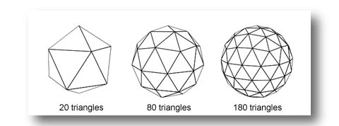
Geometry rendering depends most directly on the polygon complexity of the scene. If youve built your model out of many small polygons, then you can easily drag down your frame rate as a result. Where do small polygons come from? They often come from shapes that are smooth or partially smooth like spheres and cylinders. Without telling you, your modeler may be tesselating your sphere object into hundreds of polygons. Unless you need to zoom into such a sphere, youll never need more than about 80 polygons to make a really nice looking sphere (thats still a lot for just one object!). Consider how big the object will usually be in terms of pixels rendered on the screen. If its screen size is usually going to be quite small, then maybe the user wont even notice the difference between a sphere and a tetrahedron, and the later would save enormously on polygons.
How many total polygons is a good number? This depends on your hardware, of course, but environments that use more than 1000 polygons at any one time may not be well suited for real-time requirements. If your polygon count is very high, consider lowering the tesselation level, replacing polygon density with textures (discussed in the "Applying Textures" topic), using level-of-detail (LOD) nodes (coming soon), or developing your own scene database to manage objects. Even adding fog to your scene can be an easy way to let you render less and give the illusion that objects far away are just obscured by low visibility.
Texture rendering depends on how many pixels must be "painted" to fully render a scene. In a very simple scene, with no overlapping polygons, the number of rendered pixels will not exceed the product of your screens horizontal times vertical dimensions. For instance, a 640 x 480 screen has 307K pixels, each one of which must be cleared and then redrawn every frame update. A good graphics card these days can paint about 75M pixels per second. That means it can redraw the screen at 244 Hz if theres absolutely nothing else going on. Handling geometry, even just a few hundred polygons, plus other rendering tasks typically brings your realized performance down by 50%. Still, 122 Hz is great. Now, add stereo and render the scene twice every graphics update (one for each eyepoint), and the frame rates drops to 61 Hzjust at the edge of the maximum rate that a typical HMD can display. Unfortunately, frame rate usually drops still further for the following reason. If instead of non-overlapping polygons, the scene contains overlapping polygons, the computer actually draws that much more just to solve the hidden surface removal problem.
A simple example is rendering a cube from the inside. No matter where the viewpoint is turned to, there will never be overlapped polygons even though the total number of polygons in view may change. Consider what happens if the viewpoint is stepped back out of the cube while aimed towards the cubes center. Just as the viewpoint pierces the cubes wall, only one polygon will be in view and it will fill the whole screen. No big deal, right? Wrong! Suddenly now, behind that polygon are 5 others that together also fill the whole screen. The fact that these 5 are hidden doesnt change the fact that they get rendered. So, to continue with the calculations started above, if the frame rate was 61 Hz while instead the cube, then it will then drop to 30 Hz as soon as the viewpoint moves outside. You now see how hard it can be to maintain a high frame rate.
To avoid the pixel rendering penalty, be careful how you design your environments and avoid overlapping polygons anywhere you can. You can also take advantage of back-face culling which is a technique that allows the renderer can eliminate polygons whose front faces dont point toward the observer. This solves the problem of viewing a cube from the outside, but as soon as you move into the interior all polygon faces would be pointed away and there would be nothing to see (since they would be "culled"). The "tut_box.wrl" will demonstrate this if you load it into VRUT and move the eyepoint in and out.