Case Matching Software Vignette
Try the case matching web app (no R needed).
1) Using the Case Match Software in R
In this section I illustrate the different features of the case match software. For convenience, I expand upon the examples used in my paper "Case Selection via Matching".
As noted in the paper, I use the case match software to identify pairs of similar EU and non-EU cases based on Mahalanobis distance calculated for five variables (see Table 2). The variables are political freedom, civil liberties, GDP per capita, trade, and socialism.
To run the case match function, there is a need to define an ID variable (variable that identifies unique cases) and the matching variables. The function also allows one to define treatment and outcome variables. Note that the function offers certain flexibility where these variables can be defined before running the function, or within the function.
# Load Data from package caseMatch
library(caseMatch)
data(EU)
## Define matching variables
mvars <- c("socialist","rgdpc","FHc","FHp","trade")
# Define the "leftover" variables in the dataset to not include in the matching
dropvars <- c("countryname", "population", "eu")
a) Match using all Cases
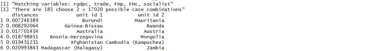
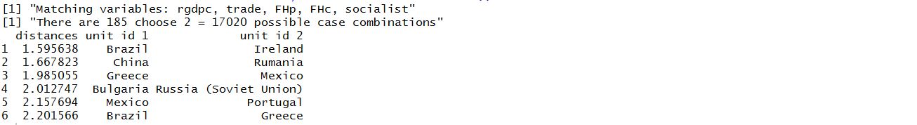
The most basic use of the case match function is to search the whole dataset for the best possible matches for all units (ignoring EU status), in a most similar design.
Note that the function case.match() requires several inputs. First, the function needs to understand the structure of the data. Thus, the function takes in the original data (data=EU), the ID variable (id.var=="countryname") and the “discarded” data (leavout.vars=dropvars). Note that the function indirectly identifies the matching variables by excluding from the full dataset the “discarded” variables. Second, the user can specify the matching distance to use (Mahalanobis), the type of design (similar cases), the number of matches for each case (2), and the number of matches to report (50).
After running the function, the function prints automatically the top 6 matches. It will also report the number of possible case combinations, and will report if observations were removed due to missing data.
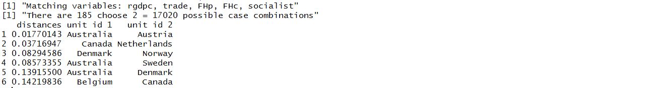
Let’s say the goal of the researcher was to estimate the impact of X (EU membership) on Y (political structures), while matching cases for important covariates (Z). Thus, instead of finding the best matches across all cases, we want cases with contrasting EU membership status.
Note that we define the treatment variable as EU membership (treatment.var=”eu”). Also, since EU membership is a binary 0/1 variable, by maximizing variance on the treatment, the function will prioritize matches between EU members (EU=1) and non-EU members (EU=0).
Sometimes the results from the matching procedure can be surprising. For instance, certain non EU countries (such as Switzerland) do not match well with other EU countries. In order to assess why, it is possible to rerun the analysis using different combinations of matching variables.
Note that the function runs each time in a loop, excluding a different matching variable each time, then records how well Switzerland matches. The results indicate that that if we took out trade or GDP, Switzerland would match better. This indicates that Switzerland matches poorly because it has a combination of trade and GDP per capita that is relatively far from others in the data.
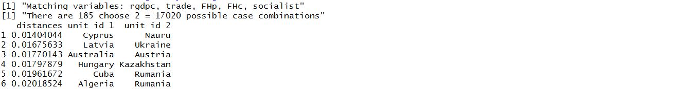
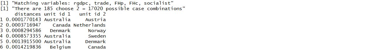
A user may decide that they want to give more or less weight to some of the matching variables. In our example, the user may want to see how matches change, depending on the relative weight one assigns to economic or political factors.
We can easily change the weights – this time upweight the political variables.
By comparing the output, we see that the matches are not sensitive to the choice of weights. This implies that the cases match well on both economic and political factors.
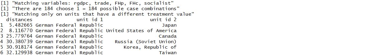
The case match function allows users to find matches for a specific case. To see this, let’s search for the best non-EU matches for Germany. Note that we match on a specific case by adding to the function (match.case=”Germany Federal Republic”).
Note that the function only finds matches for Germany. The results suggest that Japan is best non EU match for Germany.
Let’s say the user was interested in pursuing other forms of case selection (see Seawright and Gerring 2008), such as exploratory (hypothesis identification - identify X by matching on the outcome and covariates) or to identify causal mechanisms (identify a causal mechanism by matching on X, the outcome, and covariates). To do so, the case match software allows the user to match on the outcome variable.
Note that we match on an outcome variable by specifying an outcome variable (outcome.var=”population”) and to prioritize matches between countries with different population sizes. In this case, we may be able to identify causal mechanisms by matching between EU and non-EU countries, while focusing on countries with very different population sizes.
In this section, I provide possible ways to illustrate the results provided by the case match software.
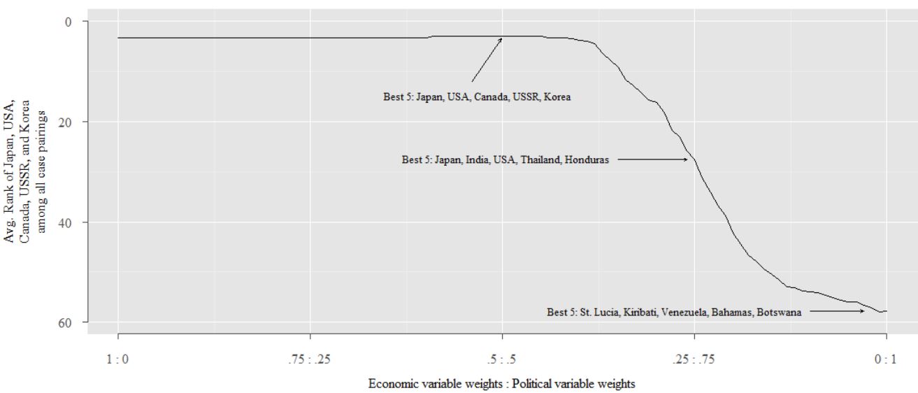
First, I replicate Figure 1 from my paper. To recap, the figure shows the average rank of the 5 best matches for Germany, over different weighting schemes. As noted in the paper, the results in Figure 1 show that the case selection depends on the relative weight assigned to economic and political variables. The economic variables appear to dominate, so the top matches are stable as long as at least 40 percent of the weight is on economic variables. However, if the political variables are weighted highly, then the matches change substantially. The original matches move far down the list, while other cases take their place at the top.
To create this figure, I create a loop which loops through different weighting schemes. I then record the average rank of the top 5 non-EU matches for Germany when there are no weights (Japan, USA, Canada, USSR, and Korea), and the top 5 matches for every given weight scheme.
Note that the “plain” output indicates that the matches are pretty stable until political variables are weighted highly. To make the output a little nicer, one can use the following R code.
## Run the matching:
## I'm not matching a specific case.
out <- (case.match(data=EU, id.var="countryname", leaveout.vars=dropvars,
                    distance="mahalanobis", case.N=2,
                    number.of.matches.to.return=10))
out$cases
b) Contrast on a key variable
out2 <- (case.match(data=EU, id.var="countryname", leaveout.vars=dropvars,
                   distance="mahalanobis", case.N=2,
                   number.of.matches.to.return=10,
                   treatment.var="eu", max.variance=TRUE))
c) Different Matching Variables
holder <- rep(NA,length(mvars))
names(holder) <- mvars
for(i in 1:length(mvars)){
  tmpdropvars <- c(dropvars,mvars[i])
  tmptab1 <- (case.match(data=EU, id.var="countryname", leaveout.vars=tmpdropvars,
                         distance="mahalanobis", case.N=2,
                         number.of.matches.to.return=200,
                         treatment.var="eu",max.variance=TRUE))$cases
  holder[i] <- min(as.numeric(rownames(tmptab1[tmptab1[,2]=="Switzerland" | tmptab1[,3]=="Switzerland",])),
                   na.rm=T)
  ## If we take out trade, it's the eighth best match
}
holder

d) Variable Weights
# Weights
# Need to make sure that the names line up
myvarweights <- rep(1, length(mvars))
names(myvarweights) <-names(dat)[-which(names(dat)%in% c(idvar, dropvars))]
print(myvarweights)
# "rgdpc"     "trade"     "FHp"       "FHc"       "socialist"

## Find the best matches while downweighting political variables:
myvarweights<-c(1,1, 0.1, 0.1, 0.1)


economic<-(case.match(data=EU, id.var="countryname", leaveout.vars=dropvars,
                    distance="mahalanobis", case.N=2,
                    number.of.matches.to.return=10,
                    treatment.var="eu", max.variance=TRUE,
                    varweights=myvarweights))
## this time with variable weights that upweight political variables:
myvarweights<-c(0.1,0.1, 1, 0.9, 0.8)
political<-(case.match(data=EU, id.var="countryname", leaveout.vars=dropvars,
                      distance="mahalanobis", case.N=2,
                      number.of.matches.to.return=10,
                      treatment.var="eu", max.variance=TRUE,
                      varweights=myvarweights))
e) Find Matches for a Specific Case
tabGer <- case.match(data=EU, match.case="German Federal Republic",
                     id.var="countryname", leaveout.vars=dropvars,
                     distance="mahalanobis", case.N=2,
                     number.of.matches.to.return=10,
                     treatment.var="eu", max.variance=TRUE)
f) Other Types of Case Selection
# Other forms of case selection

outcome <- (case.match(data=EU, id.var="countryname", leaveout.vars=dropvars,
                      distance="mahalanobis", case.N=2,
                      number.of.matches.to.return=10,
                      treatment.var="eu", outcome.var="population",
                      max.variance=TRUE, max.variance.outcome=TRUE))
2) Visualization
## Match germany with different variable weights
myvarweights <- c(1,1,.1,.1,.1)
## make a sequence of weights
ws <- seq(0,1,.01)
## Compare to top 5
top5 <- as.character(tabGer$cases[,3])[1:5]
## make holders
robustholder1 <- list()
robustholder2 <- rep(NA,length(ws))
## loop over the weights, running the matching each time
for(i in 1:length(ws)){
print(i)
myvarweights <- c(ws[i],ws[i],(1-ws[i]),(1-ws[i]),(1-ws[i]))
tmpGer <- (case.match(data=EU, match.case="German Federal Republic",
id.var="countryname",leaveout.vars=dropvars,
distance="mahalanobis", case.N=2,
number.of.matches.to.return=200,
treatment.var="eu", max.variance=TRUE,
varweights=myvarweights))
matchesGer <- as.character(na.omit(tmpGer$cases)[,3])
robustholder2[i] <- mean(which(matchesGer %in% top5))
robustholder1[[i]] <- matchesGer[1:5]
}
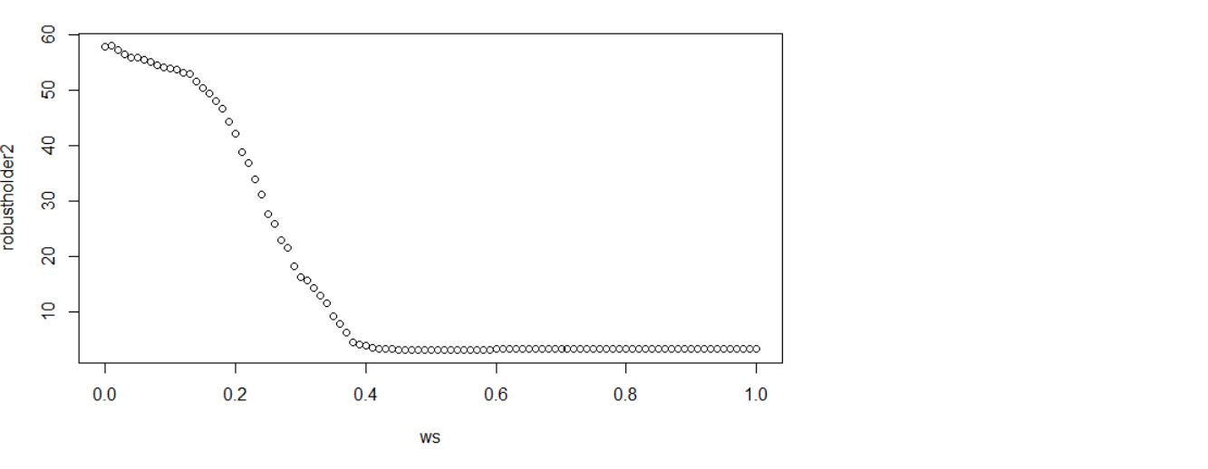
plot(ws, robustholder2)
## make a plot for the paper
pdf("EU.pdf",6.8,3.7)
par(mar=c(3.7,5.8,.5,.5), family="serif")
plot(ws, robustholder2,type="n",axes=F,xlab="",ylab="",ylim=c(60,0))
polygon(x=c(-10,10,10,-10),y=c(-1000,-1000,1000,1000),col="gray90")
pp <- par()
ss <- c(0,.25,.5,.75,1)
abline(v=ss,col="white")
midss <- sapply((1:(length(ss)-1)),function(i){mean(c(ss[i+1],ss[i]))})
abline(v=midss,col="#ffffff50")
ss <- c(0,20,40,60)
abline(h=ss,col="white")
midss <- sapply((1:(length(ss)-1)),function(i){mean(c(ss[i+1],ss[i]))})
abline(h=midss,col="#ffffff50")
axis(1,at=c(0,.25,.5,.75,1),labels=c("1 : 0",".75 : .25",".5 : .5",".25 : .75","0 : 1"),
col="gray30",col.axis="gray30",las=1,tck = -0.015)
axis(2,at=c(0,20,40,60),labels=T,col="gray30",col.axis="gray30",las=1,tck = -0.015)
title(xlab="Economic variable weights : Political variable weights", line=2.5)
title(ylab="Avg. Rank of Japan, USA,\nCanada, USSR, and Korea\namong all case pairings",line=2.5)
lines(ws,rev(robustholder2))
## add top 5 cases at various points
robustholder1[[50]]
ws[50]
text(.6,15,"Best 5: Japan, USA, Canada, USSR, Korea",pos=2,cex=.8)
arrows(x0=.46,y0=12,x1=.498,y1=3.5, length=.04)
##
robustholder1[[1]]
ws[1]
text(.9,58,"Best 5: St. Lucia, Kiribati, Venezuela, Bahamas, Botswana",pos=2,cex=.8)
arrows(x0=.9,y0=57.8,x1=.97,y1=57.8, length=.04)
##
robustholder1[[26]]
robustholder2[26]
ws[26]
text(.65,27.6,"Best 5: Japan, India, USA, Thailand, Honduras",pos=2,cex=.8)
arrows(x0=.65,y0=27.6,x1=.74,y1=27.6, length=.04)
##
dev.off()
End