Tensors are powerful mathematical objects with wide-ranging applications in physics, from elastic mechanics and general relativity to modern developments in quantum information theory and machine learning. However, their notation and representation often vary across contexts, making it difficult to recognize the underlying connections between different approaches. In this post, we offer a structured mathematical perspective and explore multiple representations of tensors, providing a systematic exposition of the different notations used in tensor analysis.

Real Tensors

Duality of Basis

Tensors over a vector space \( \mathbb{V} \) are elements of the tensor product space \( \mathbb{V}^{\otimes n} \), constructed by taking \( n \) copies of \( \mathbb{V} \) and combining them via the tensor product. To describe tensors quantitatively, we choose a basis, a set of linearly independent vectors that spans \( \mathbb{V} \). Once a basis is fixed, tensors can be expressed in terms of their components, which are the coefficients associated with each basis element. For example, a vector (a rank 1 tensor) can be written as \[ \mathbf{u} = u^1 \mathbf{g}_1 + u^2 \mathbf{g}_2, \] where \( \{\mathbf{g}_1, \mathbf{g}_2\} \) is a basis for \( \mathbb{V} \), and \( \{u_1, u_2\} \) are the corresponding components of \( \mathbf{u} \). Similarly, a rank 2 tensor can be written as \[ \mathbf{T} = T^{ij}\mathbf{g}_i\mathbf{g}_j, \] where \( T^{ij} \) are the components of \( \mathbf{T} \) in the chosen basis, and repeated indices imply summation (Einstein summation convention). Although the choice of basis is arbitrary, the tensor itself remains invariant. It represents the same geometric or physical object regardless of the basis used for its description. This invariance will be an important theme in our following discussion.

However, the basis we have chosen is not necessarily orthonormal under a given inner product. To account for this, we define a dual basis. Given a basis \(\{\mathbf{g}^i\}\), we introduce another set of basis vectors \(\{\mathbf{g}_i\}\), which is defined by the condition \[ \mathbf{g}^i \cdot \mathbf{g}_j = \delta^i_j. \] These two sets of basis vectors are known as the contravariant and covariant bases. For consistency, contravariant bases are denoted with upper indices, while covariant bases are denoted with lower indices.

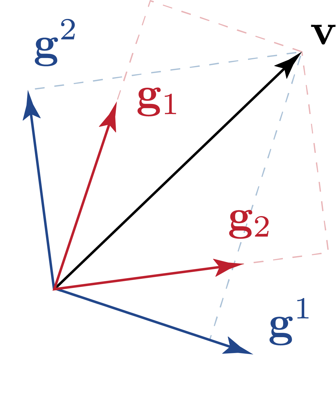
We use the Gram matrix, \(g_{ij}\), to lower and raise indices, as it defines the relationship between the basis vectors in a given space. The Gram matrix can also be understood as components of the metric tensor, expressed as \( I = g_{ij} \mathbf{g}^i \mathbf{g}^j = \delta^i_{\cdot j} \mathbf{g}_i \mathbf{g}^j= \delta_i^{\cdot j}\mathbf{g}^i \mathbf{g}_j\). Explicitly, the Gram matrix is given by \[ g_{ij} = \mathbf{g}_i \cdot \mathbf{g}_j = (g^{ij})^{-1}.\] where \[ g^{ij} = \mathbf{g}^i \cdot \mathbf{g}^j.\] The relationship between covariant and contravariant basis vectors corresponds to raising and lowering indices: \[ \mathbf{g}^i = g^{ij} \mathbf{g}_j \] for raising an index, and \[ \mathbf{g}_i = g_{ij} \mathbf{g}^j \] for lowering an index. A similar transformation applies to vector components, where the contravariant and covariant components are related by \( u^i = g^{ij} u_j \) and \( u_i = g_{ij} u^j \).

Active Transformation

In an active transformation, the transformation is affected by a linear map \(\mathcal{A}\). For simplicity, we assume that \(\mathcal{A}\) is invertible and maps between vector spaces \(\mathbb{U}\) and \(\mathbb{U}^\prime\). The vector \(\mathbf{u}\in\mathbb{U}\) is taken to a new vector \(\mathbf{u}_A^\prime\in\mathbb{U}^\prime\) by applying the linear map \(\mathcal{A}\). The components of the new vector are denoted as \({u^\prime}^i\), and in order to describe the transformation, we introduce a set of coefficients \(\beta^i_{\cdot j}\). The forward and inverse transformation rules are listed on the right, with the inverse of the transformation matrix denoted as \(\left(\beta^{-1}\right)^i_{\cdot j}\).

Passive Transformation

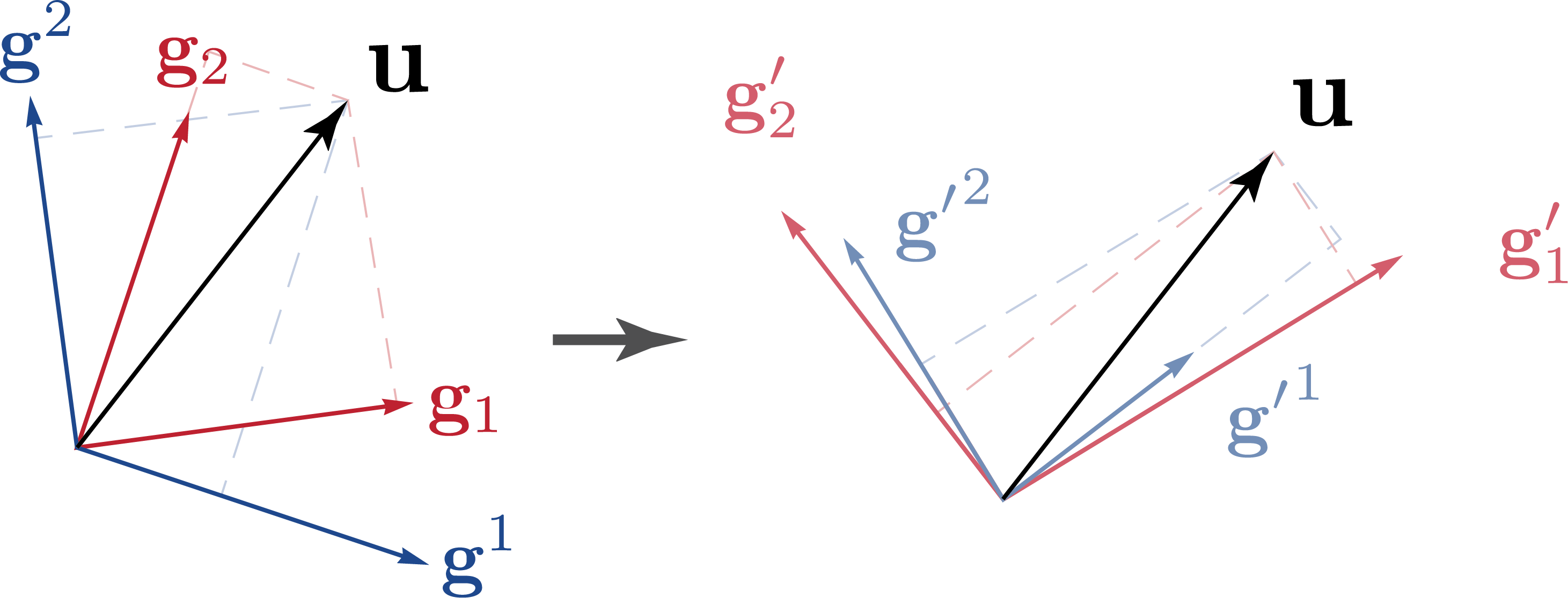
Passive transformations provide an alternative perspective: the same vector is represented in a different basis without altering the vector itself. This is especially useful when describing a physical system from different perspectives.

More precisely, we keep the tensor \(\mathbf{u}\) fixed while expressing its components with respect to a new basis. \[\mathbf{u} = u^i\mathbf{g}_i = u_i \mathbf{g}_i = {u^\prime}^i \mathbf{g^\prime}_i = u^\prime_i \mathbf{g^\prime}^i\] For consistency, we adopt the convention that the components \(u^i\) transform in the same way as in the active transformation.

The transformation and inverse transformation rules for the basis vectors and components are shown on the right, totalling 8 rules, expressed in the same coefficients \(\beta^i_j\) as those defined in the active trasnformation. These rules are derived by first assuming one of them, for instance, \(u^{\prime i}=\beta^i_ju^j\). By expressing \(\mathbf{u}\) in two different ways, \(\beta^i_{\cdot j}u^j\mathbf{g}^\prime_i=u^j\beta^i_{\cdot j}\mathbf{g}^\prime_i\), we can compare both expressions and deduce \(\mathbf{g}_i = \beta_{\cdot i}^{j} \mathbf{g^\prime}_j\). There are four such relations, each conneting a basis transformation rule to a component transformation rule. The fact that four of the rules are the inverses of the other four further organizes the eight transformation rules into two distinct groups. One additional relation is needed to establish a connection between these two groups. Namely, we can express the coefficients in two ways using the derived rules, \((\beta^{-1})_{\cdot i} ^j = \mathbf{g^\prime}_i \cdot \mathbf{g}^j = \mathbf{g}_i\cdot\mathbf{g}^{j^\prime}\) to link them. However, there is one drawback with this notation: Since \(u^{\prime i}\) denotes the component of \(\mathbf{u}\) in the new basis instead of the original basis, it doesn't hold true that \(u_i^\prime=\beta_{\cdot i}^j u_j\) as if we were to naivly raise and lower the indices.

To resolve this visual inconsistency, it is customary to use the alternative notation for coordinate transformation rules. Namely, instead of using a prime as a superscript to indicate transformed quantities (e.g., \(\mathbf{g}^\prime_i\)), we place the prime directly on the index itself, such as \(\mathbf{g}_{i^\prime}\). This notation explicitly associates the transformation with the index rather than the entire tensor, making it clearer which basis the components are expressed in. Additionally, since we will be able to tell whether \(\beta\) is inverted based on the placement of the \(\prime\), we omit the explicit inverse notation to further simplify the notation.

We can also relate the new metric tensor to the old one using the transformation coefficients. As we will see later, this is a special case of the more general transformation rules of rank 2 tensors.

Finally, for the special case when \({\mathbf{e}^i}\) is a set of orthonormal basis, the metric tensor is \[g^{ij} = \mathbf{e}^i \cdot \mathbf{e}^j = \delta^{ij}\]

Relation Between the Two Transformations

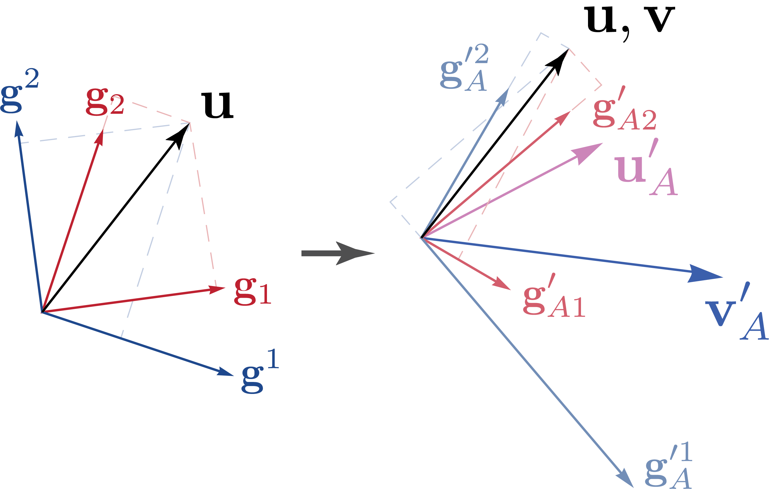
To further contrast the differeces between the active and passive transformations, we introduce a set of transformed basis \(\mathbf{g}_{A\ i}\) under the active transformation \(\mathbf{g}^\prime_{A\ i}=\mathcal{A}(\mathbf{g}_i)\). With it, the transformed vector can also be expressed as \(\mathbf{u}_A^\prime = u^i \mathbf{g}_{A\ i}^\prime\). That is, to maintain consistency with the component transformations, the basis vectors must transform inversely to how they do in the passive transformation. We can further define the dual map of the active transformation. Specifically, the transformation is affected by the linear map corresponding to the inverse adjoint of the primal transformation, \(\mathcal{A}^{\star -1}\). To distinguish it from vectors that transform under the primal transformation \(\mathbf{u}\to\mathbf{u}^\prime_A\), we denote a generic dual vector by \(\mathbf{v}\), which transforms to \(\mathbf{v}^\prime_A\) under the dual map. This specific choice ensures that the transformed primal and dual bases are still dual to each other. The extended active transformation rules are shown on the right.

Matrix Representation

We also provide the exact form of the matrix corresponding to the transformation coefficients \(\beta\). The transformation matrix is defined as \[ [B] = \begin{bmatrix} & & \\ &\beta^i_{\cdot j}& \\ & & \end{bmatrix},\] with \(i\) representing the row index and \(j\) representing the column index. Explicitly writing out everything in their matrix form, the transformation rules for the basis under passive transformations are expressed as:

The transformation rule summarized in the box on the right.

Transformation Rules of Rank 2 Tensors

A tensor (element of a tensor product space \(V^{\otimes 2}\)) can also be expressed in terms of a basis and its components, which obey the transformation rules above. For example, a rank 2 tensor can be written as: \[\mathbf{T} = T^i_{\cdot j} \mathbf{g}_i \mathbf{g}^j = T^{ij} \mathbf{g}_i \mathbf{g}_j = T_i^{\cdot j} \mathbf{g}^i \mathbf{g}_j = T_{ij} \mathbf{g}^i \mathbf{g}^j\] The tensor transpose is defined by swapping the order of the basis vectors: \[\mathbf{T}^{\tau} = T^i_{\cdot j} \mathbf{g}^j \mathbf{g}_i = T^j_{\cdot i} \mathbf{g}^i \mathbf{g}_j = (T^{\tau})_i^{\cdot j} \mathbf{g}^i \mathbf{g}_j,\] where \((T^{\tau})_i^{\cdot j} = T^j_{\cdot i} \). Since the operation is defined without specifying any explicit coordinate, it defines a coordinate invariant, or canonical, operation. In comparison, the matrix transposition will give rise to \([T^i_{\cdot j}]^T=[T^j_{\cdot i}]\). This demonstrates the relationship between the tensor transpose and the matrix transpose: For components such as \([T^{ij}]\) or \([T_{ij}]\), taking the tensor transpose is equivalent to taking the matrix transpose; however, for mixed-type components, such as \([T_i^{\cdot j}]\), this does not necessarily hold true.

Coordinate Transformation as Contraction

For real tensors, the linear map associated with the active transformation can be interpreted as a contraction with a second-rank tensor, denoted by \(\mathbf{A} \cdot\) Similarly, the transformation of the basis can be written in tensor notation as: \[\mathbf{g^\prime}_i = \mathbf{A} \cdot \mathbf{g}_i.\] What are the explicit forms of the tensor \(\mathbf{A}\)? It turns out we can define \(\mathbf{A}\) in terms of the old and new bases as well, as shown in the box.

Complex Tensors

Passive Transformation

For complex tensors, the transformation rules have to be slighly modified. Yet still, similar to the real case, we can derive the passive transformation relations by expressing the components of \(u\), or more commonly in quantum information as \(\ket{u}\), in the new basis: \[\mathbf{u} = \overline{u^i}\mathbf{g}_i = \overline{u_i}\mathbf{g}^i = \overline{u^{\prime i}} \mathbf{g^\prime}_i = \overline{u^\prime_i} \mathbf{g^\prime}^i\] Here, the components are denoted as their complex conjugates to ensure that the transformation rules of the components and the bases are apparently the same.

This differs from the usual convention in quantum mechanics, where the components are typically taken to be unconjugated. For example, \( \ket{u} = u^i \ket{g_i} \). To match that convention, one would need to conjugate all coefficients when applying the \( u \)-rules. Here, however, we adhere to the original (mathematical) convention rather than the one commonly used in physics.

Another main difference to note is the transformation rules of the dual vectors, this is because the duality map is no longer linear, but sesquilinear. Suppose we are looking at a dual vector \( \langle v^i \mathbf{g}_i,\cdot \rangle = \overline{v^i} \langle \mathbf{g}_i,\cdot \rangle \). The transformation rules for the \( v \) coefficients will differ from those of \( u \), in the same way as in the physics convention. To determine which transformation rules apply (whether the component belongs to a bra or a ket), we will need a way to label the components. We will use dotted notation for the indices. For a basis vector of the dual space (bra) or a component of a ket, we place a dot underneath the index, such as \( \underset{\cdot}{i} \). With the dotted notation, the transformation rules are shown on the right. A easy mnemonic for this rule is to conjugate the \(\beta\) coefficiets whenever the dot is on the bottom.

Active Transformation

In active transformation, the new vector can be expressed similarly, with the components involving complex conjugation: \[\mathbf{u}_A^\prime = \overline{u^i}\mathbf{g^\prime}_i = \overline{{u^\prime}^i} \mathbf{g}_i,\] with the component transformation rules identical to those in passive transformation.

Tensor Representation

However, the tensor transpose can still be defined for complex tensors. There are two sets of tensors that are commonly used. One of them is those operators belonging to \(V^{\lor}\otimes V\). \[\mathbf{T} = \overline{T^{\underset{\cdot}{i}}_{\cdot j}} \mathbf{g}_i \mathbf{g}^\underset{\cdot}{j} = \overline{T^{\underset{\cdot}{i}j}} \mathbf{g}_i \mathbf{g}_\underset{\cdot}{j} = \overline{T_{\underset{\cdot}{i}}^{\cdot j}} \mathbf{g}^i \mathbf{g}_\underset{\cdot}{j} = \overline{T_{\underset{\cdot}{i}j}} \mathbf{g}^i\mathbf{g}^\underset{\cdot}{j} \] The other is an element of \(V^{\otimes 2}\): \[\mathbf{\Psi} = \overline{\Psi^i_{\cdot j}} \mathbf{g}_i \mathbf{g}^j = \overline{\Psi^{ij}} \mathbf{g}_i \mathbf{g}_j = \overline{\Psi_i^{\cdot j}} \mathbf{g}^i \mathbf{g}_j = \overline{\Psi_{ij}} \mathbf{g}^i \mathbf{g}^j\] To transform the components to the new basis, we simply apply the corresponding rules for the rank 1 case. For instance, \(T_{i^\prime}^{\cdot\underset{\cdot}{j^\prime}}=\beta^{\underset{\cdot}{i}}_{i^\prime}\beta_{j}^{\underset{\cdot}{j^\prime}}T_{i}^{\cdot\underset{\cdot}{j}}\), and \(\Psi_{\underset{\cdot}{i}^\prime}^{\cdot\underset{\cdot}{j^\prime}}=\overline{\beta^{i}_{\underset{\cdot}{i^\prime}}}\beta_{j}^{\underset{\cdot}{j^\prime}}\Psi_{\underset{\cdot}{i}}^{\cdot\underset{\cdot}{j}}\) The tensor adjoint operation (analogous to the tensor transpoose in the real case) is defined by swapping the order of the basis vectors and conjugating the components. \[\mathbf{T}^{\star} = T^i_{\cdot \underset{\cdot}{j}} \mathbf{g}^j \mathbf{g}_\underset{\cdot}{i}.\] As it turns out, the adjoint is coordinat independent as it can be written as a composition of \(\flat \circ \mathcal{T}^{\lor} \circ \sharp\) even tensor transposition cannot be defined in a canonical fashion.