Textbook expositions often begin with the BB84 protocol and build up from there to establish its security. In contrast, we will take a top-down approach. We'll start by clearly defining the underlying quantum information task and then introduce a more powerful tool—entanglement distillation—as a conceptual framework for solving it. Through a series of reduction, this perspective will lead us back to the BB84 protocol.

Task Definition and Security Measure

Task Definition

In classical cryptography, we can use a one-time pad to achieve secure communicaation through a public channel provided we share a resource \([cc]_{\text{priv}}\). This corresponds to the resource inequality:

\[ [cc]_{\text{priv}} + [c \rightarrow c] \geq [c \rightarrow c]_{\text{priv}} \]

To generate \([cc]_{\text{priv}}\), we can use classical cryptographical methods, such as one way functions that requires superpolynomial time to compute. However, this requires the extra assumption that eve's computing power is bounded. But we can overcome this issue with the aid of quantum mechanical principles. Specifically, quantum key distribution (QKD) allows us to generate a shared private key between two parties (Alice and Bob) that is secure even against an adversary with quantum capabilities. This level of security is known as unconditional security.

One of the brute-froce strategies to QKD is to first prepare shared entanglement (entanglement distribution). Due to the monogamy of entanglement, the two parties can obtain a shared secret bit by measuring both branches of the EPR pair. \[ [qq] \geq [cc]_{\text{priv}} \] This may seem to be an overkill, but we will soon see that a protocol that performs entanglement distribution can be reduced to one that performs only QKD under a series of simplification. More precisely, our goal is to obtain \([qq]\) even in the presence of an adversary, with suitable success probability and finite rate. We begin with an entanglement-based QKD protocol (Lo-Chau), then reduce it to the standard BB84 protocol.

Security Definition

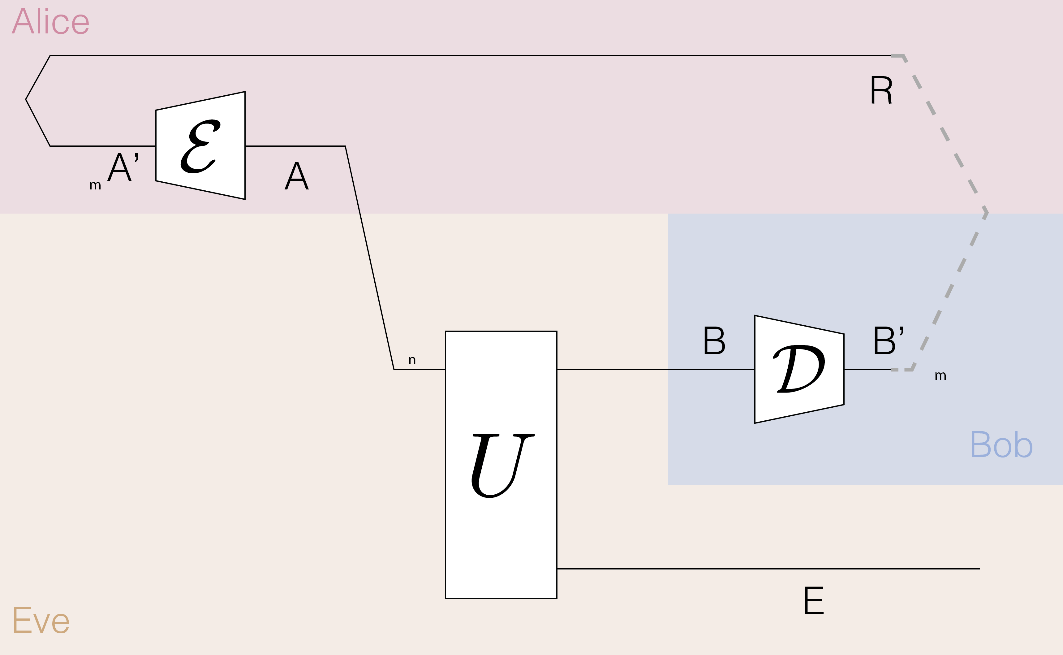
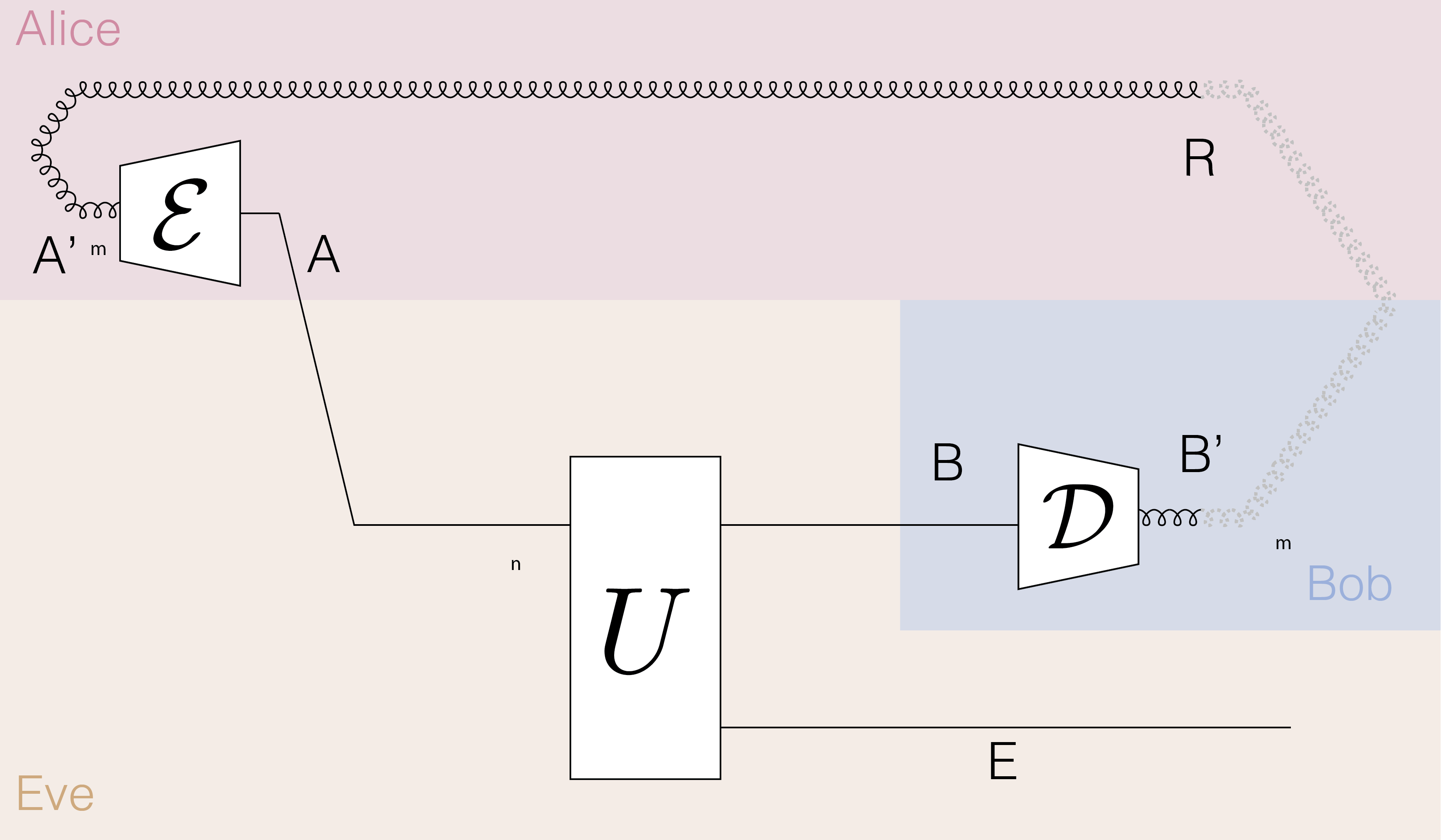
We now specify some parameters of the protocol. First, we have three parties: Alice, Bob, and Eve. Alice and Bob are connected by a public quantum channel \(\mathcal{N}_{A^\prime \to B^\prime}\) acting on \(n\) qubits, and Eve is assumed to have unlimited access to the channel—meaning that she can, in the worst case, access the full purification of the channel, denoted by an isometric extension \(U_{A\to BE}\). Note that we do not assume the channel is i.i.d. We assume that Alice and Bob each have \(m\) subregisters. Alice can apply an encoding map \(\mathcal{E}_{A \to A^\prime}\), and Bob can apply a decoding map \(\mathcal{D}_{B^\prime \to B}\), potentially assisted by a classical side channel. In distribution protocols, it is natural to include an additional reference system \(R\) to purify Alice’s input state. This will be useful for defining the figure of merit.

In entanglement distribution, the goal is to share EPR pairs between the communicating parties. We will benchmark the performance of the protocol using the trace distance between the state \(\rho_{RB^\prime}\) and \(m\) perfect Bell pairs. Alternatively, we can use the entanglement fidelity \(F_E\) as a figure of merit. The entanglement fidelity of a quantum channel \(\mathcal{N}\) with respect to the EPR state \(|\mathrm{EPR}\rangle\) is defined as \[ F_E := \langle \mathrm{EPR} | \mathcal{N_{A^\prime\to B^\prime}} (|\mathrm{EPR}\rangle\langle \mathrm{EPR}|_{AE}) | \mathrm{EPR} \rangle, \]

Once we have a functional entanglement distribution protocol, we can promote it to a QKD protocol: after Alice and Bob share a state close to ideal EPR pairs, they both measure in the \(Z\) basis to extract a classical key \(K\). Let us denote the resulting classical registers as \(K_R\) and \(K_B\) for Alice and Bob, respectively. By the monogamy of entanglement, if Alice and Bob are nearly maximally entangled, we expect \(K_R = K_B\)^[1], and furthermore, that they are nearly uncorrelated with Eve. To be more specific, suppose a bipartite state \(\rho_{AB}\) has its subsystem \(A\) being close to a pure state. I.e. \(\|\rho_A-\psi_A\|\leq \epsilon\). Converting this bound to a Fidelity bound by the FV inequality then using Ulhmann's theorem, we can show that some purification \(\phi_{ABC}\) of \(\rho_{AB}\) is close to that of the pure state \(\ket{\psi}_A\otimes\ket{\upsilon}_{BC}\). Tracing out register \(C\) and using DPI gives us the desired bound. This motivates the following definition of security:

• Completeness: If there is little interferrence from the adversary, then the protocol should succeed with high probability ^[2].
• Correctness: When the protocol does not abort, the classical outcomes form a shared key: \(K_R = K_B\).
• Secrecy: After tracing out register B, Alice's register is maximally mixed and uncorrelated with Eve: \(\rho_{KE} \approx\frac{\mathbb{I}_K}{d}\rho_E\).

The decopling criterion implies that Eve has limited Холево information: \[ I(K,E) = H(E) - H(E|K). \]

Since Alice’s key is uniform by construction, we can apply the Alicki–Fannes-Winter (AFW) inequality to bound Eve’s information about the key. Note that the converse also holds: by Pinsker’s inequality, \[ \frac{1}{2} \left\| \rho_{KE} - \frac{\mathbb{I}_K}{d}\rho_E \right\|_1^2 \leq D_{\mathrm{KL}}\left(\rho_{KE} \left\| \frac{\mathbb{I}_K}{d} \rho_E\right.\right) = I(K , E) \leq \varepsilon, \] where the \(K\) register holds the maximally mixed state. This connects trace distance closeness to Eve’s information leakage.

Some earlier works defined security using the classical mutual information between Eve’s measurement outcome and the key, which can be optimized over all POVM's of Eve to obtain the Accessible information. This is a weaker notion of security. Nevertheless, in the asymptotic i.i.d. setting, both definitions yield the same key rate. This equivalence justifies using the stronger definition without loss of generality in the asymptotic regime.

CSS Lo-Chau Protocol

Reduction to i.i.d attack

In the Lo–Chau protocol, we assume a worst-case adversary: Eve performs a coherent attack, interacting jointly with all transmitted qubits and holding a purification of the global state. This makes the joint state \(\rho_{A^m B^m E}\) highly correlated and generally non-i.i.d. across all \(m\) rounds. However, by applying a random permutation to the registers after encoding and before decoding, and invoking an exponential quantum de Finetti theorem, the reduced state on a subset of the systems becomes approximately a convex combination of i.i.d. states. Since the approximation error decays exponentially in the number of discarded subsystems, only a negligible fraction needs to be sacrificed to achieve a small trace distance error. This allows us to reduce the security analysis to collective attacks, where Eve interacts with each signal independently but may defer her measurement to the end and perform a joint POVM.

Reduction to Pauli attack

The next important reduction is the observation that we do not need to know the exact form of the i.i.d. noise affecting the shared state. Suppose Alice and Bob share \(n\) copies of some arbitrary bipartite state \(\rho_{AB}\). It turns out that for the purposes of analyzing fidelity under standard QKD protocols using stabilizer codes, we may assume without loss of generality that \(\rho_{AB}\) is Bell-diagonal. This is because, when using a standard encoder–decoder pair for stabilizer codes, the final fidelity after decoding is identical to what it would be if the input state were the corresponding Bell-diagonal state obtained by dephasing \(\rho_{AB}\) in the Bell basis. The reason is as follows. Consider an error term in \(\rho_{AB}\) of the form \(K_i \mathrm{EPR} K_i^\dagger\), where \(K_i\) is a Kraus operator from Eve’s noise channel \(\mathcal{N}\). Since the Pauli operators form a complete basis for quantum operations, each \(K_i\) can be decomposed into a linear combination of Paulis. This decomposition includes both diagonal and cross terms — for example, terms like \(X \mathrm{EPR} Z\). Under the action of the encoding and decoding circuits (e.g., unitaries of a stabilizer code), such cross terms evolve as \(U_\mathcal{R} (X \mathrm{EPR}Z) U_\mathcal{R}^\dagger\) and syndromes are measured accordingly. After decoding, each term results in either a perfect EPR pair (when the error is correctly identified and corrected) or a Pauli-rotated EPR pair orthogonal to the ideal one (when the correction fails). Importantly, these orthogonal error states do not count into the final fidelity \(F_E\), and cross terms vanish when computing \(F_E\) as well. Thus, only the diagonal terms contribute to the output fidelity.

Sifting and error estimationn

Even though we may assume the shared state \(\rho_{AB}\) is Bell-diagonal, we still don’t know the exact Bell coefficients. To estimate them, we apply the sifting trick: we randomly sample \(n/2\) of the shared pairs and measure them in the \(XX\) basis and the other \(n/2\) in the \(ZZ\) basis. These measurements are destructive (they will measure \(ZI\), \(IZ\)), but by the law of large numbers, we can accurately estimate the effective error rates with high probability—thanks to the i.i.d. assumption.

Reducing error parameters

An even simpler approach is to perform an \(H\)-twirl, where we apply random Hadamard gates to the shared qubits before measurement. This operation symmetrizes the state, mapping it to one where the \(X\) and \(Z\) error components are averaged (e.g., \(p_X = p_Z\)). In this case, it suffices to estimate the error rate in just one basis, such as the \(XX\) basis.

Even if \(X\) and \(Z\) errors are correlated, this does not affect the analysis, since the case with independent \(X\) and \(Z\) errors represents the worst-case scenario. When applying independent decoders for bit-flip and phase-flip errors, the logical \(X\) and \(Z\) failure rates remain unchanged, even though the logical \(Y\) failure rate may differ. If the observed error rates fall below the channel's threshold, the protocol proceeds with entanglement purification followed by privacy amplification to extract a secure final key.

Alternatively, we can perform a \(2\pi/3\) twirl in the \(\frac{1}{\sqrt{3}}\left(\hat{\mathbf{x}}+\hat{\mathbf{y}}+\hat{\mathbf{z}}\right)\) direction. This transforms the state into a Werner-like form with equal error probabilities in all three Pauli directions: \(p_X = p_Y = p_Z\). This enables us to correct the errror with a capacity-achieving code for depolarizing noise.

Quantum error correction (Private amplification and information reconciliation)

To perform quantum error correction non-locally on \(n\) EPR pairs, we begin by noting that each pair is stabilized by the operators \(Z_{iA} Z_{iB}\) and \(X_{iA} X_{iB}\). These stabilizers can be mapped, via a symplectic change of basis, into the standard stabilizer code structure consisting of stabilizers \(S_{iA} S_{iB}\), destabilizers \(D_{iA} D_{iB}\), and logical operators \(\overline{X}_{jA} \overline{X}_{jB}\), \(\overline{Z}_{jA} \overline{Z}_{jB}\). In this new basis, errors on Bob’s half (branch \(B\)) can be detected by jointly measuring the stabilizers \(S_{iA} S_{iB}\), which are symmetric between Alice and Bob. These can be measured destructively on both sides. Alice then sends her measurement outcomes \(S_{iA}\) over the public classical channel, enabling Bob to compute the full syndrome and apply the appropriate correction. Once error correction is complete, Alice and Bob can decode within the logical subspace to extract the purified state. Although in our previous discussion we assumed the stabilizer measurements were non-destructive, this distinction does not affect the outcome. Since the syndrome space is ultimately traced out during decoding, whether the measurement is destructive or not has no impact on the final fidelity \(F_E\).

Key generation thresholds

By Shannon theory, we know that random CSS codes asymptotically saturate the hashing bound. In the case of independent bit-flip and phase-flip errors, the achievable rate is given by \[ R = 1 - h_b(p_X) - h_b(p_Z), \] where \(h_b\) denotes the binary entropy function and \(x, z\) are the respective \(X\) and \(Z\) error rates. For the special case of \(H\)-twirled states, where \(p_X = p_Z\), this simplifies to \[ R = 1 - 2 h_b(p_X), \] yielding a threshold at \(p_X \approx 0.11\). For Werner-like (i.e., fully depolarized Bell-diagonal) states, we can go further: by using general stabilizer codes instead of CSS codes, we can saturate the full Pauli hashing bound \[ R = 1 - H(p_I, p_X, p_Y, p_Z), \] where \(p_I = 1 - p\), and \(p_X = p_Y = p_Z = p/3\) represent the probabilities for the three Pauli errors. This gives a higher threshold, with the secure key extraction possible up to \(p_X=2p/3 \approx 0.126\).

Protocol Steps

The resulting key is provably secure under the assumption that quantum mechanics holds and that the error rates remain below threshold. This forms the entanglement-based basis of BB84, which we discuss next.

Reduction to BB84

Overview of CSS code

Let \( C_X, C_Z \leq \mathbb{F}_2^n \) be classical linear codes such that \[ C_Z^\perp \leq C_X \quad \text{(equivalently, } C_X^\perp \leq C_Z \text{)}. \]

Define \( \dim(C_Z) = k_1 \), \( \dim(C_X^\perp) = k_2 \). Then the dimension of the quantum codespace is \[ k = k_1 - k_2. \]

Logical Operators

• Logical \( \bar{X} \) operators live in the quotient space: \(C_Z / C_X^\perp.\)
• Logical \( \bar{Z} \) operators live in the quotient space: \( C_X / C_Z^\perp. \)

We can always pick the logical operators such that logical \(X\)'s only consist of \(X\) operators, and logical \(Z\)'s only consist of \(Z\) operators.

Destabilizers

We can also define destabilizers. For instance, \( X \)-type destabilizers must anticommute with \( Z \)-type stabilizers, which come from \( C_Z^\perp \), so they must lie outside \( C_Z \). Therefore they live in: \(\mathbb{F}_2^n / C_Z ,\) and can be made purely \(X\).

Definition: Codeword in \( C_Z / C_X^\perp \)

The logical states of the CSS code is in one-to-one correspondence to the elements of the quotient group \( C_Z / C_X^\perp \). For every element \(x\), we define the respective codeword \(\ket{x}=\ket{x+C_X^\perp}\). For a destabilizer state with destabilizer \(D_X\) and \(D_Z\), \(\ket{x,d_X,d_Z}=\sum_{c\in C_X^\perp}(-1)^{c \cdot d_z}\ket{x+c+d_X}\).

Removal of Alice's measurement and \(X\) basis information

Since Alice will measure her EPR pairs eventually, we can simply let her encode the other half of the states in random logical codewords with random destabilier values, i.e., \(\ket{x,d_X,d_Z}\). Moreover, since Bob only needs the Z-type stabilizer info, we can average out the X-type information on Alice's side to start with. This results in a mixed state \(\sum_{c\in C_X^\perp}\ket{x+d_X+c}\bra{x+d_X+c}\). This can be alternatively reinterpreted as Alice simply sending out random bits, and later she extracts the \(d_X\) and \(x\) information.

Removal of the need of QRAM

Instead of having Bob wait until Alice to tell him the correct basis to measure in, we can let him measure in a random basis as soon as he receives the qubits. This will result in half of the basis being wrong, so we will have to start with \(4n\) insead of \(2n\) qubits.

Removal of permutation

Since we can use a permuted version of the error correcting code each time, and also randomize our sampling qubits, we won't have to use the explicit permutation. With the above reductions, we finally arrive at the original BB84 protocol:

Protocol Steps