Qōan Blog

This blog post delves into the graphical representation of tensor analysis, focusing on applications in quantum mechanics and quantum information theory.

Vectors and EPR states

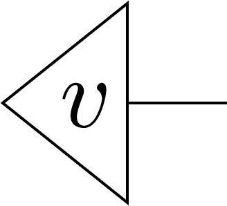
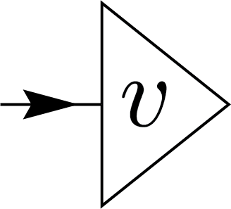
Tensor network notation is a visual and compact way to represent complex mathematical objects, such as tensors, and their interconnections in a graphical form. In tensor network notation, a vector is represented as a triangle with a single line extending from one of its sides. For example, the vector \(\mathbf{v}\) can be depicted as on the right.

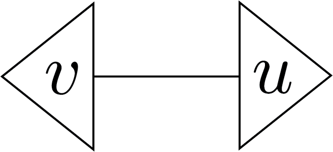
The inner product of two vectors, \( \mathbf{v} \) and \(\mathbf{u}\), \(\mathbf{v} \cdot \mathbf{u} = v_i u_i\), can be represented as a tensor contraction in the network. This corresponds to connecting the line extending from the triangle for \( \mathbf{v} \) to the line from the triangle for \( \mathbf{u} \), indicating summation over the shared index. The fact there is not open lines means the result is a scalar value

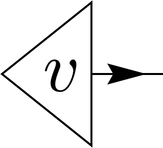
For complex vectors (kets), we can similarly represent tensor nodes as vectors. However, a challenge arises when considering the inner product, which is sesquilinear rather than linear, meaning swapping the two arguments results in complex conjugation, so it does not exhibit simple reflection symmetry. To address this, we introduce an arrow to indicate the direction in which we read the notation.

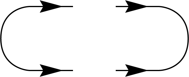
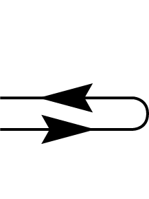
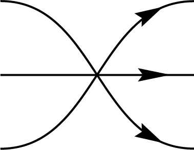
So far, we have focused on tensorial objects, which are invariant under coordinate transformations. This means their components transform covariantly when the basis changes. In quantum information theory, however, a special basis (such as the computational basis) is often used, and it can be useful to define objects specific to this basis. One example is the EPR state ^[1], which is graphically represented as two arrows pointing in opposite directions along the line. This state is defined as \( \frac{1}{\sqrt{d}}|ii\rangle \) in the computational basis. However, if we define the EPR state in a different basis, such as the \( |y; \pm \rangle \) basis in the qubit \(d=2\) case, where it is given by \( |y;+ y;+\rangle + |y;- y;-\rangle \), it corresponds a different state than the one defined in the computational basis.

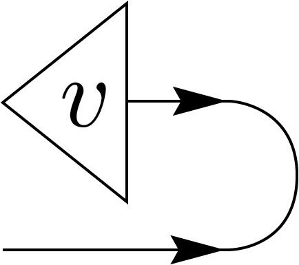
Applying the EPR state to vectors results in the transpose of the vectors. For example, in the computational basis, \(v^i\ket{i}\) is mapped to \(v^i\bra{i}\). This ensures the map is linear, but it is not canonical since the maximally engtangled is not. Also it’s not an isometric isomorphism, unlike the conjugate-linear adjoint operation that maps kets to bras ^[2].

\(=\)

\(=\)

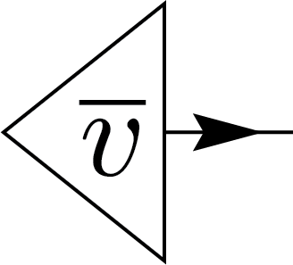
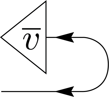
An alternative way to denote these transposed states is to incorporate noncanonical operations, such as conjugation of the components, directly into the states’ nodes as part of their labels. In this case, the node with \(\overline{v}\) denotes the ket \(\overline{v_i}\ket{i}\). We can further take the adjoint of the state by reversing the directions of the arrows and this will lead to the equalities on the left ^[3].

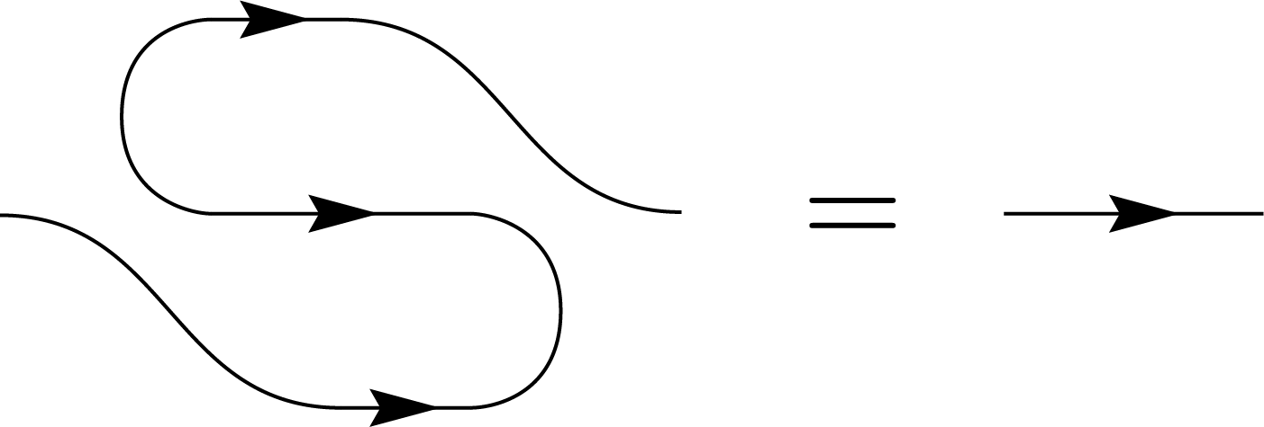
Finally, by combining two such EPR states, we can recover a canonical state, a process commonly referred to as the snake identity.

Linear operators

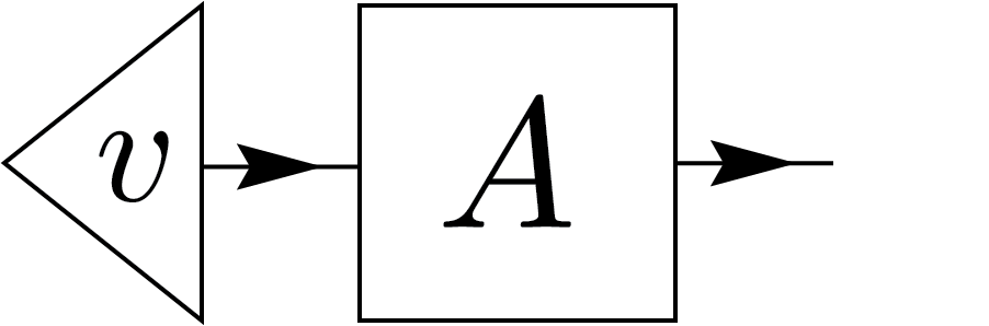
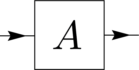
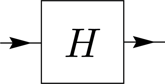
Now, we consider a linear operator that resides in the tensor product space of primary and dual spaces, naturally represented with one arrow going in and another going out. This operator acts on a vector as \( A|v\rangle \), which can also be interpreted as a quantum circuit essentially read in the direction of the arrows!

Similarly, we can apply the transposition map to operators by contracting them with EPR states on both sides. This defines the matrix transposition \( A^\top \), which, in this context, is also noncanonical but plays a crucial role in quantum information theory. This transformation can also be represented using the necklace identity.

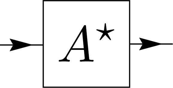
Another commonly used operation in quantum information is the Hermitian conjugate, typically denoted by the superscript \(\dagger\). However, to emphasize its role as a canonical operation, we use \(\star\) to denote the Hermitian conjugate (or adjoint, as referred to in mathematical literature), and reserve \(\dagger\) for an noncanonical matrix operation. I.e. for non-orthogonal bases, the \(\dagger\) operation is noncanonical. However, in any orthogonal basis, the matrix transposition inherent in the definition of \(\dagger\) aligns with the canonical operation denoted by \(\star\). This distinction mirrors our use of \(\top\) and \(\tau\) to differentiate between matrix transposition and tensor transposition.

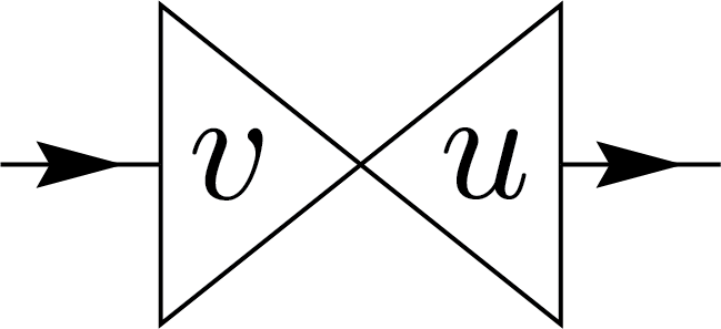
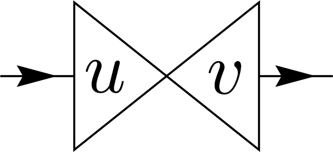
Moreover, in line with the intuition that \( A \) can be decomposed into terms like \( \ket{v} \bra{u} \) as shown on the right, and that Hermitian conjugation can be performed by swapping \( u \) and \( v,\) we may also want to reverse the direction of the arrows, determining which port serves as input and which as output. However, the square notation of the operator makes it difficult to distinguish between them.

\(=\)

\(=\)

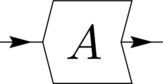
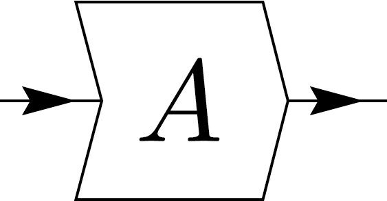
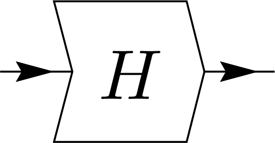
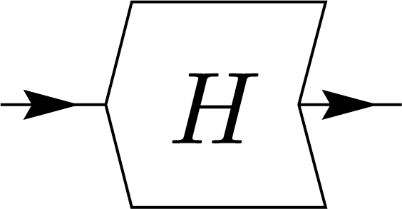
To solve this, we use a box with angled edges shaped like \(\langle\) and \(\rangle\) to indicate directionality. The inward-pointing edge \(\langle\) represents the input, while the outward-pointing edge \(\rangle\) represents the output. This design, as shown below, also allows us to express the adjoint operation simply by flipping the node. We can express Hermiticity (self-adjointness) of operators with the notation:

\(=\) \(=\)

Density matrices and Channels

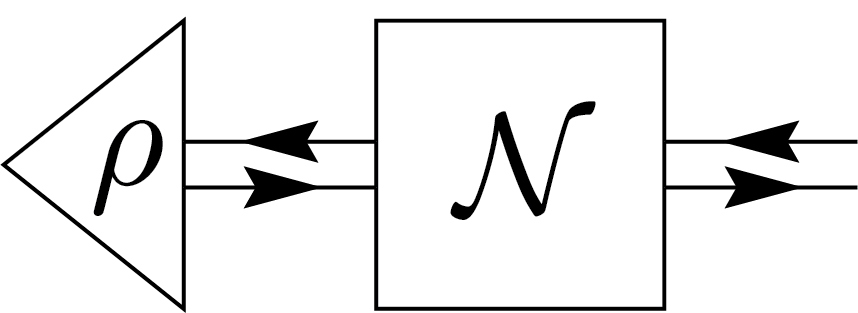
Density matrices are fundamental operators in quantum information theory, describing the statistical state of a quantum system. They are also physical in the sense that they uniquely characterize the extraction of classical data from quantum systems. These matrices are typically acted upon by conjugation when performing transformations such as unitary evolution or interactions with the environment. To simplify their representation and manipulation in diagrams, an alternative notation using double grouped lines with arrows pointing in opposite directions is often employed. Here, we use the density matrix \(\rho\) as an example to illustrate this approach. This notation should be interpreted equivalently to \(\rho\) being an operator node, with the arrows moved to a single side.

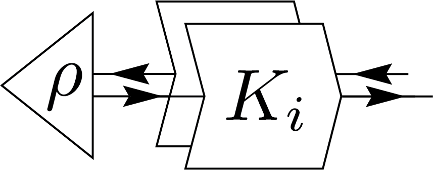
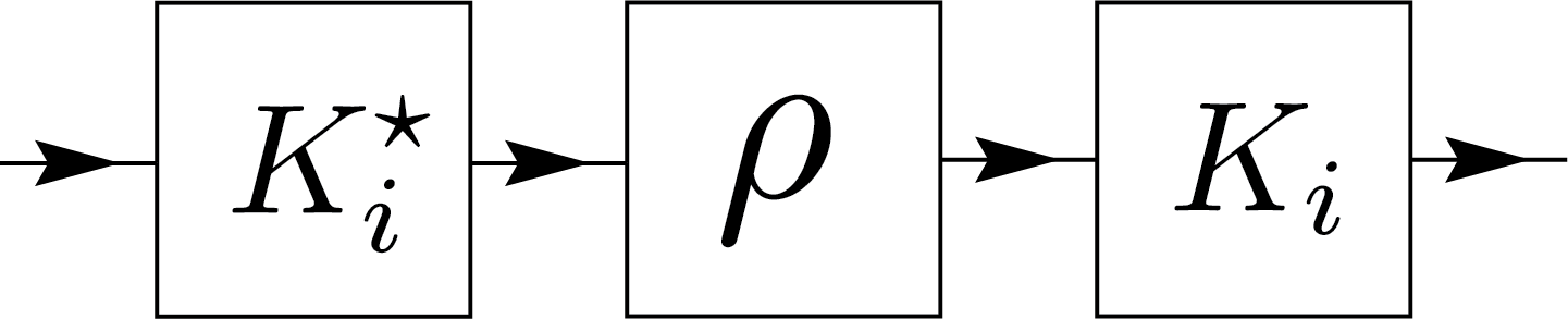
Generic quantum operations, which encompass the preparation, evolution, and measurement of quantum states, are mathematically described by quantum channels. They can also be used to capture the dynamics of open quantum systems, including both unitary evolution and the effects of noise or decoherence induced by interacting with the environment. A quantum channel, denoted as \(\mathcal{N}\), can be represented by a set of operators known as Kraus operators, \(\{K_i\}\). These operators satisfy the completeness relation \(\sum_i K_i^\dagger K_i = I\), ensuring the preservation of probabilities. Each Kraus operator \(K_i\) corresponds to a specific transformation/process that contributes to the overall effect of the channel on a quantum state. The way that \(\mathcal{N}\) acts on a state \(\rho\) is shown as:

\(=\) \(=\)

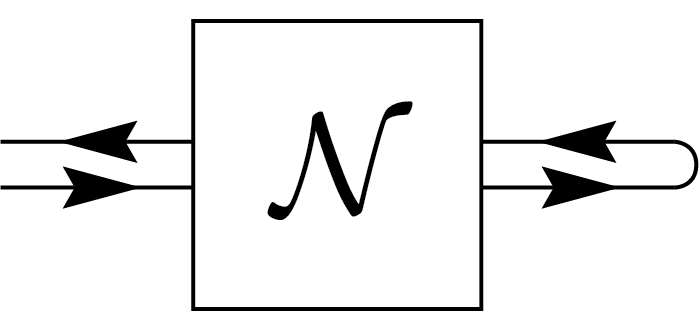
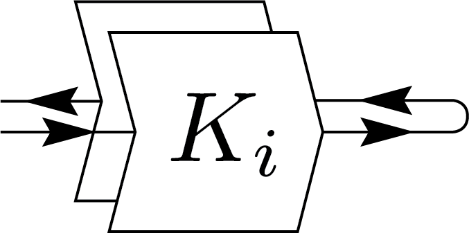
For a quantum channel to be valid, it must satisfy two conditions: complete positivity (CP) and trace preservation (TP). The TP condition can be naturally represented using graphical notation shown below.

\(=\) \(=\) \(=\)

However, the CP condition, requiring the channel to be positive semidefinite (PSD), is more challenging to express graphically because graphical representations are better suited to linear conditions. When addressing the CP condition, we often need to revert to the mathematical expressions for clarity.

Relation to Other Notations

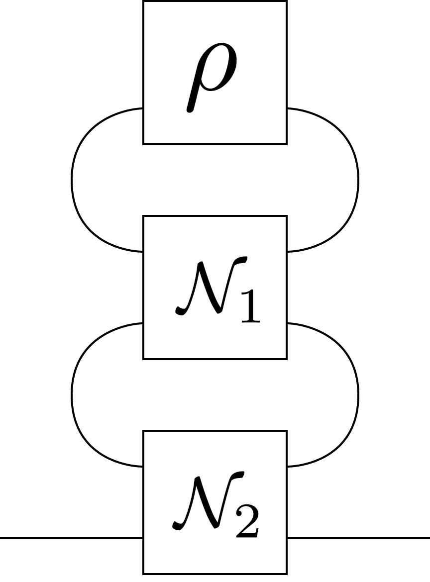
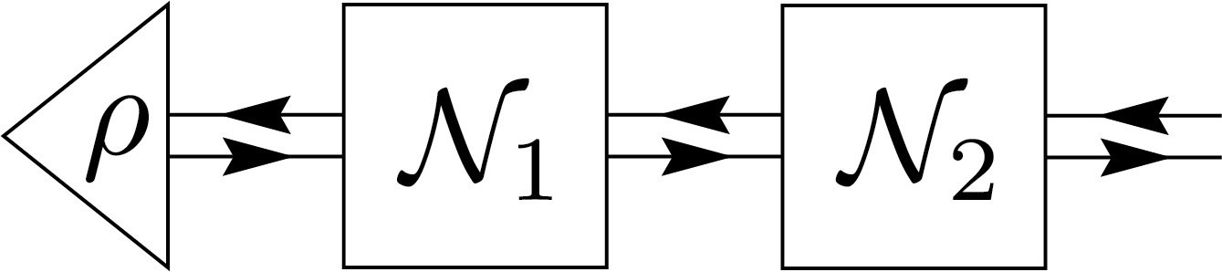
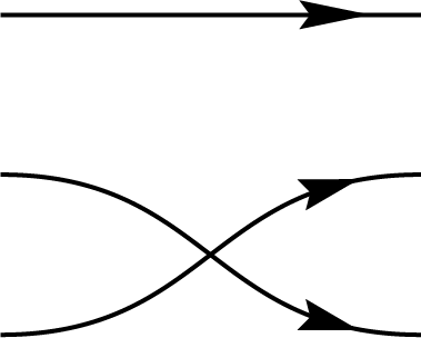
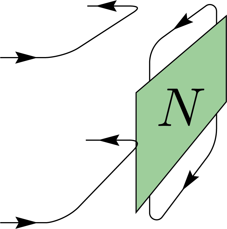
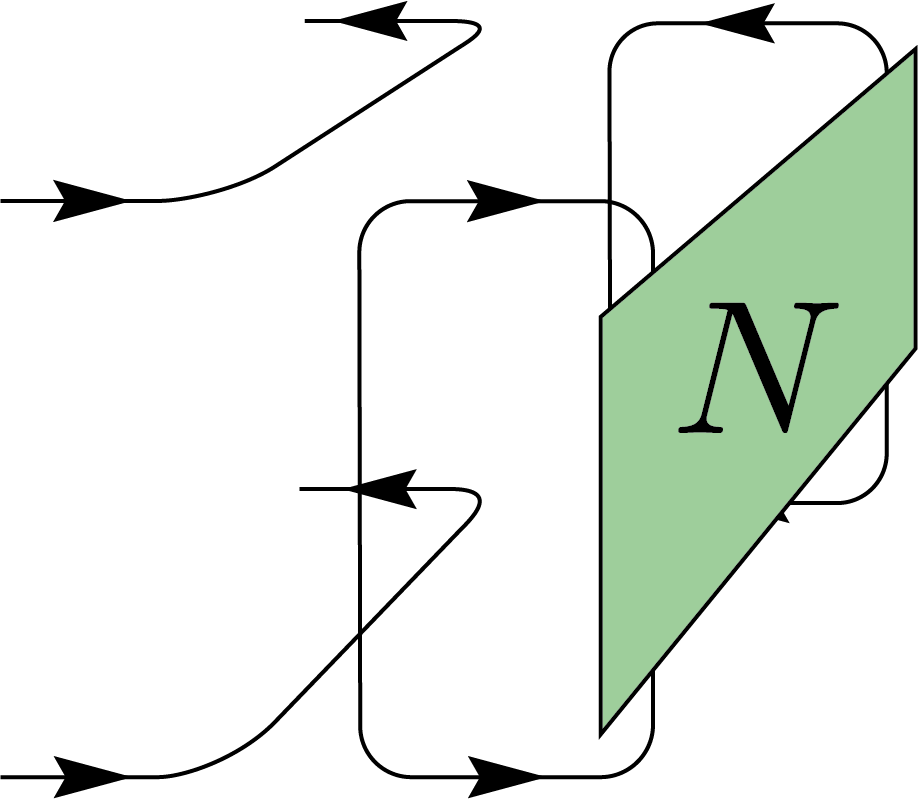
In various literature on similar topics, authors often use a notation without arrows WBC15. In undirected graphical representations, all kets correspond to open lines pointing to the right. To transition from the undirected graph to the directed graph, one simply adds right-pointing arrows to all the lines. Similarly, to revert to the undirected representation, the graph need to be first arranged such that all the arrows are pointing to the right, and then the arrows can be removed while maintaining the overall connectivity and structure of the graph. As an example, consider the following graph representing the successive application of two quantum channels \(\mathcal{N}_1\) and \(\mathcal{N}_2\) on a density matrix \(\rho\) represented in the two different notations:

\(=\)

Birdtracks

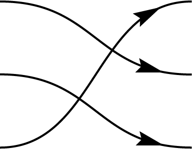
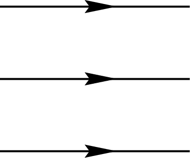
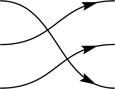
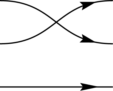
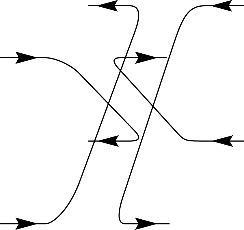
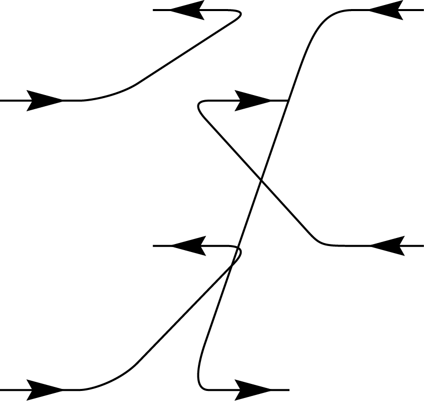
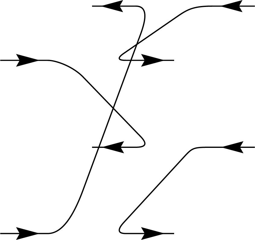
Graphical representations can be used to depict permutations between multiple registers by simply connecting the input register to the corresponding output. These diagrams are referred to as birdtracks in Alc18. For example, the permutation \((123)\), which cyclically shifts the content of register 1 to register 2, register 2 to register 3, and register 3 back to register 1, can be represented as a diagram where the first port connects to the second, the second to the third, and the third back to the first. In addition to \((123)\), there are five other permutations among three registers, collectively forming the \(S_3\) symmetric group. In this context, \(S_3\) corresponds specifically to the permutation representation on \(V^{\otimes 3}\):

\(\Biggl\{\) \(,\) \(,\) \(,\) \(,\) \(,\) \(\Biggl\}\)

Weingarten Calculus

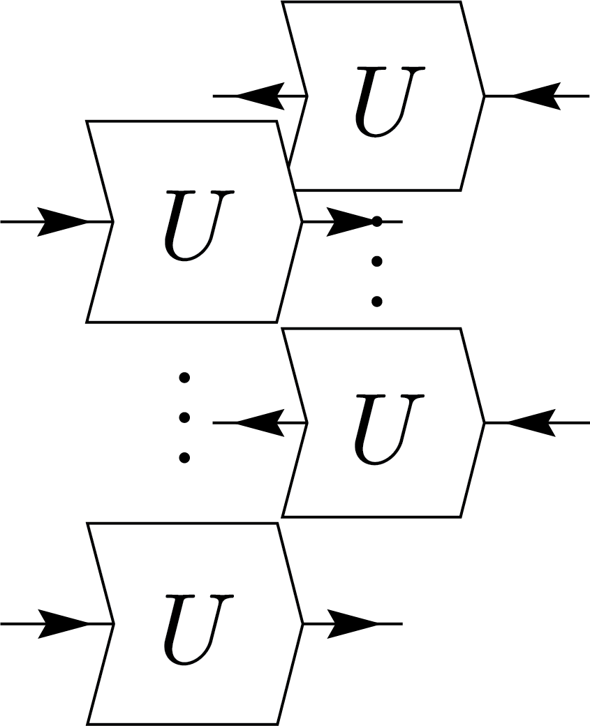
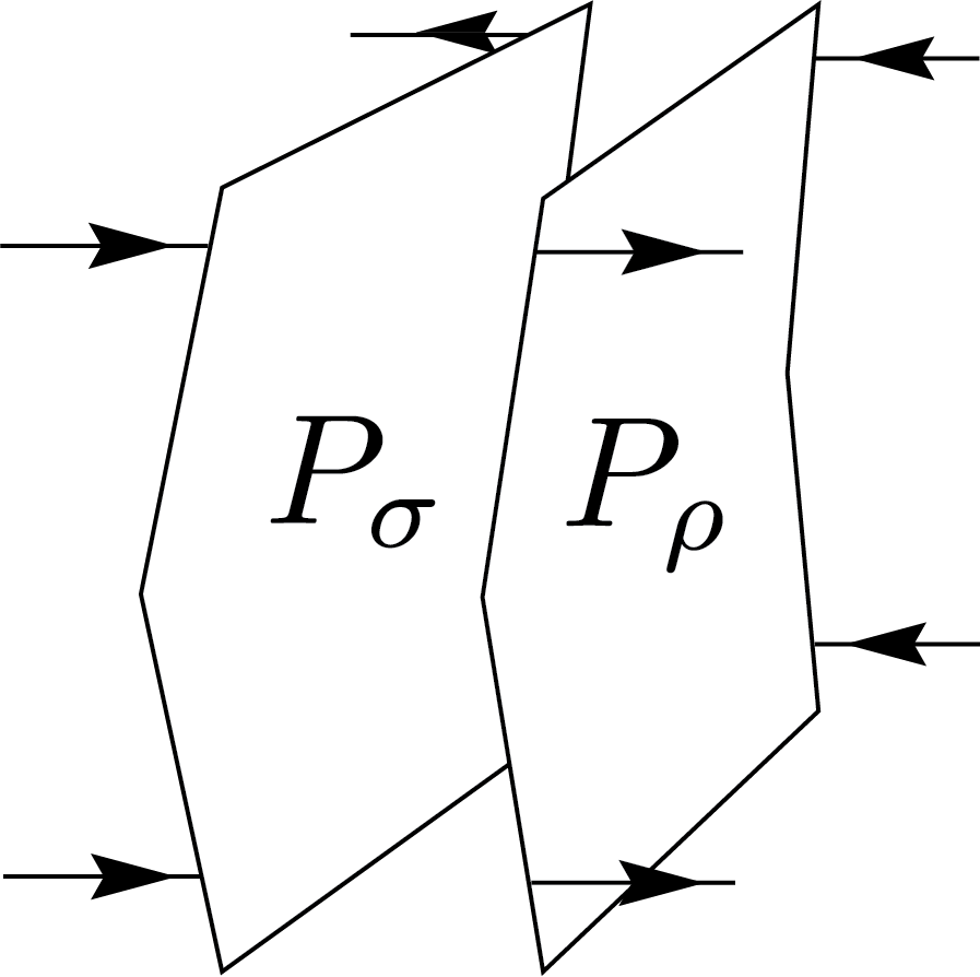
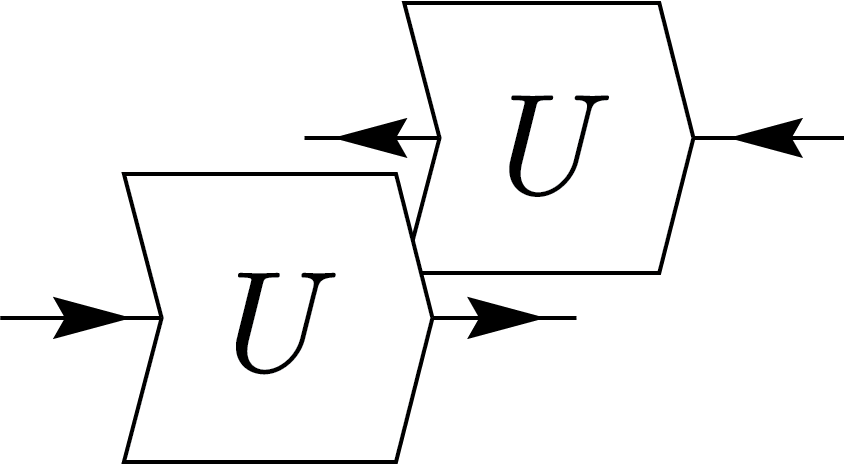
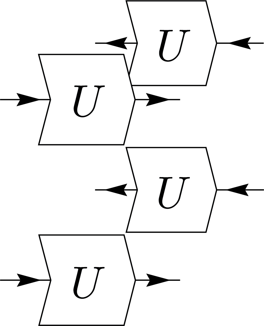
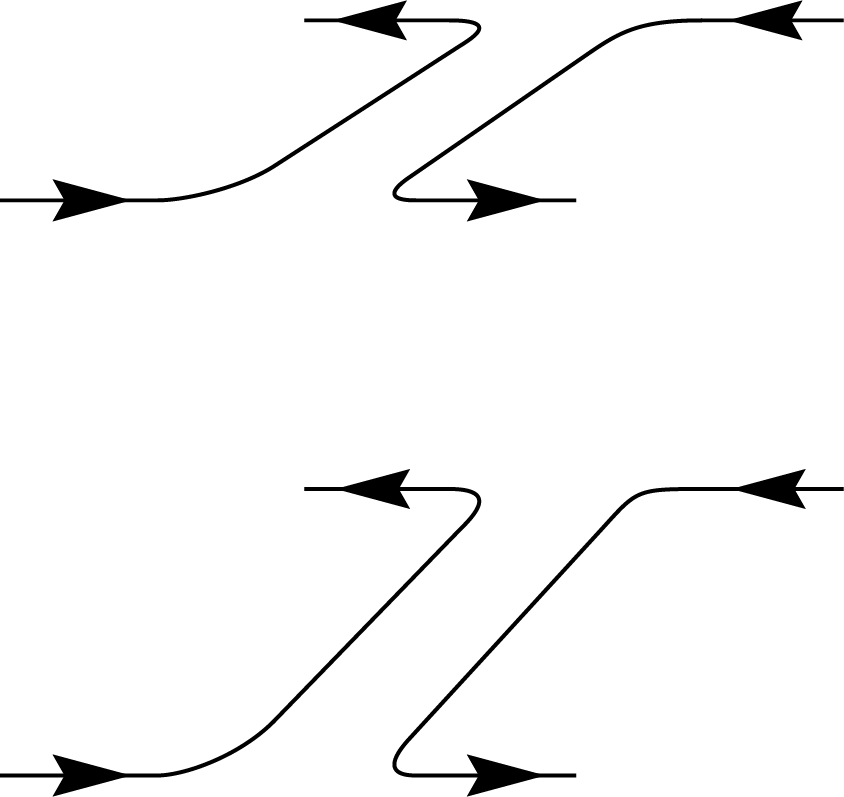
Weingarten calculus, named after physicist Donald Weingarten, provides a method for evaluating Haar-averaged tensor products of unitary matrices. Specifically, it evaluates integrals with the following equation: \[ \int_{\mu_\mathrm{Haar}} U_{i_1 j_1} \cdots U_{i_n j_n} \overline{U_{i'_1 j'_1} \cdots U_{i'_n j'_n}} = \sum_{\rho,\sigma \in S_n} W(\rho^{-1}\sigma, d) \delta_{I\,\rho(I')} \delta_{J\,\sigma(J')}. \] In other words, the result is a linear combination of permutations weighted by Weingarten functions \( W(\cdot, \cdot) \), which depend on the group elements \(\sigma\in S_n\) and the dimension \( d \). In essence, Weingarten calculus expresses Haar integrals as combinatorial sums over symmetric group elements with an elegant graphical interpretation. Graphically, this can be represented as follows:

\( \displaystyle\int\) \(=\sum_{\rho,\sigma\in S_n}W(\rho^{-1}\sigma,d)\)

For the derivation and exact expressions of the coefficients, please refer to the blog post on Schur-Weyl duality. Additionally, you may find useful details in CMN22. However, please note that the article contains some typos: on page 739, \(L_{ii^\prime jj^\prime}\) should be \(L_{iji^\prime j^\prime}\), and in Theorem 4.4, the indices \(i^\prime\) and \(j^\prime\) are missing.

Now, let us explore some simple examples. We begin with the case \(n=1\), where the integral reduces to an identity operator that connects the different registers:

\( \displaystyle\int\) \(=\dfrac{1}{d}\)

This result is used in the unitary twirling of a single-register density matrix, which simply produces the totally mixed state \(\frac{\mathbb{I}}{d}\).

This demonstrates that under unitary twirling, any state becomes proportional to the maximally mixed state, reflecting complete symmetry and loss of any initial information. Now considering the case \(n=2\). The Weingarten identity yields:

\( \displaystyle\int\) \(=\frac{1}{d^2-1}\Biggl(\) \(+\) \(\Biggl)+\frac{1}{d-d^3}\Biggl(\) \(+\) \(\Biggl)\)

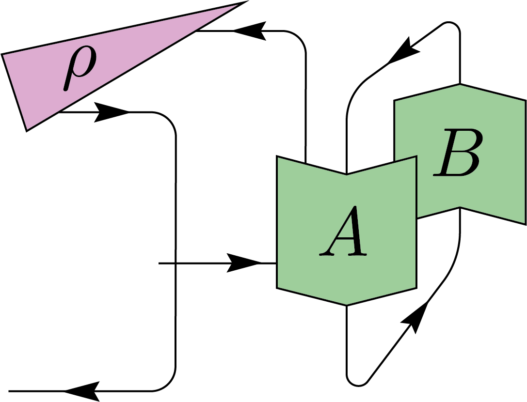
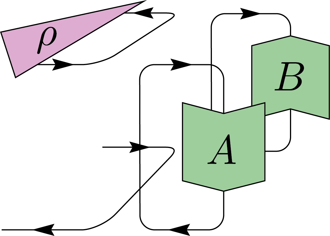
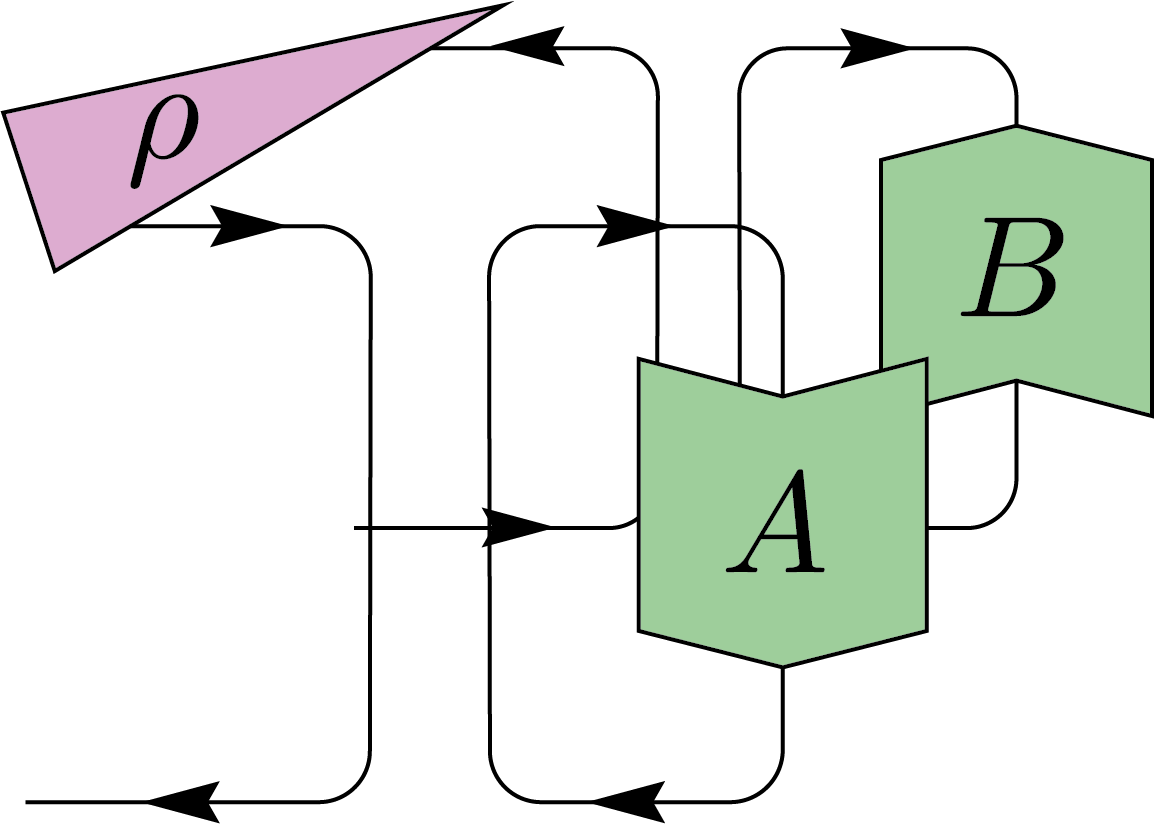
This expression involves both the identity permutation and the swap permutation within the symmetric group \(S_2\), weighted by appropriate factors depending on the dimension \(d\). We can apply this to twirl the superoperator acting on \(\rho\) of the form \(B \rho A\), where \(A\) and \(B\) are arbitrary operators. The result simplifies to:

\( \displaystyle\int\) \(=\frac{1}{d^2-1}\Biggl(\) \(+\) \(\Biggl)+\frac{1}{d-d^3}\Biggl(\) \(+\) \(\Biggl)\)

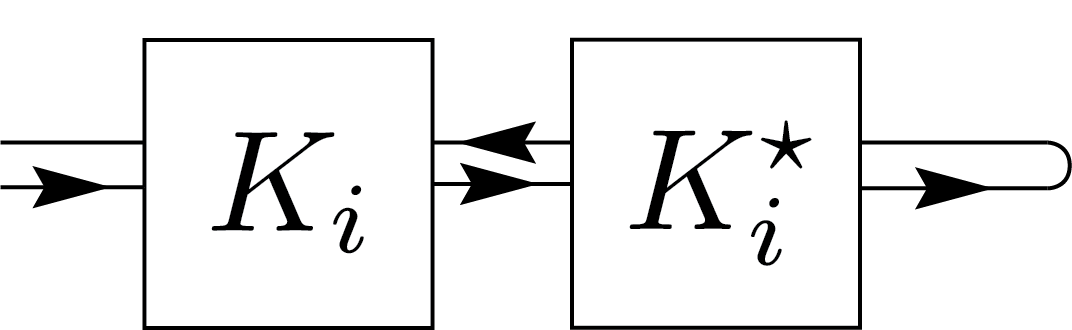
This results in an effective depolarizing channel: \[ \mathcal{D}_\lambda(\rho) = (1-\lambda)\rho + \lambda\frac{\mathbb{I}}{d}, \] where \(\lambda\), the effective depolarization parameter, is given by \[ \lambda = \frac{d\,\mathrm{tr}(AB) - \mathrm{tr}(A)\mathrm{tr}(B)}{d^2 - 1}. \] When this is a real channel, we can take \(A = K_i\) and \(B = K_i^\star\) to be the Kraus operators of a physical channel. In this case, \(\lambda\) reduces to the fidelity: \[ \lambda = \frac{d^2 - \sum_i |\mathrm{tr}(K_i)|^2}{d^2 - 1}. 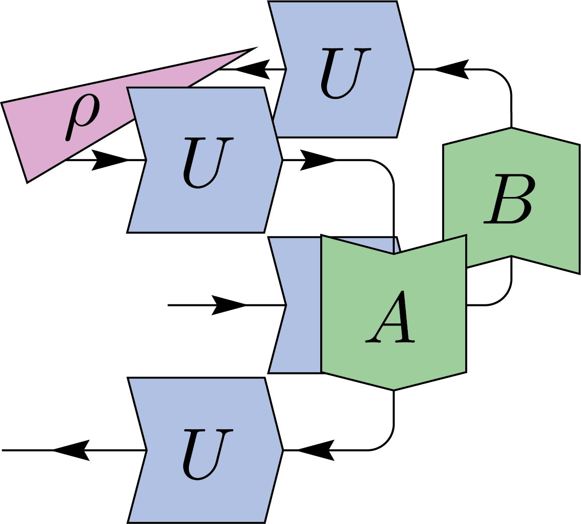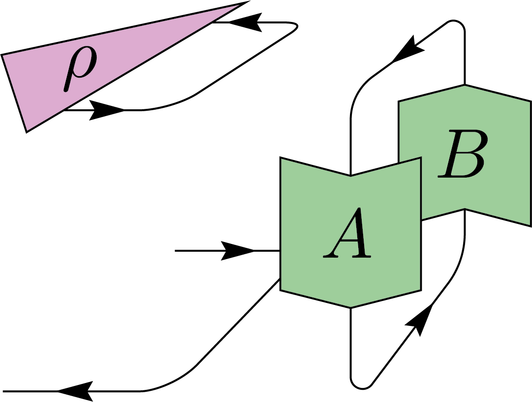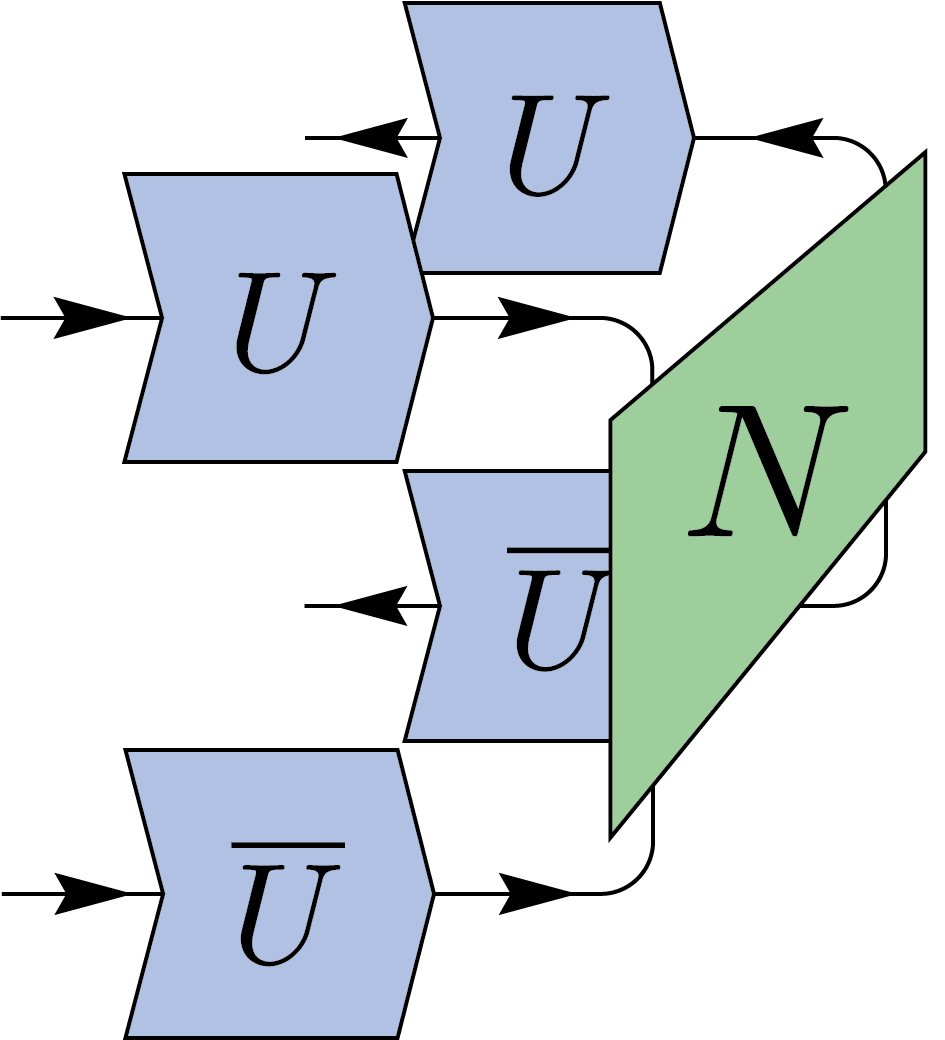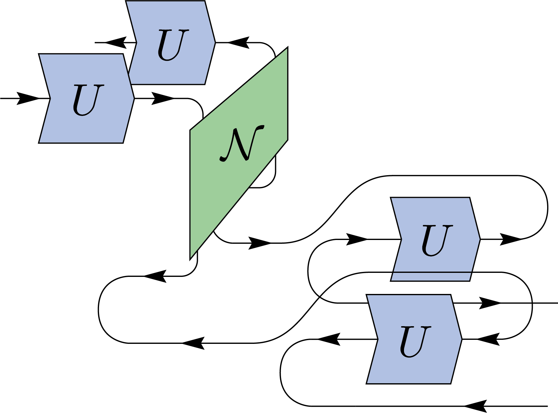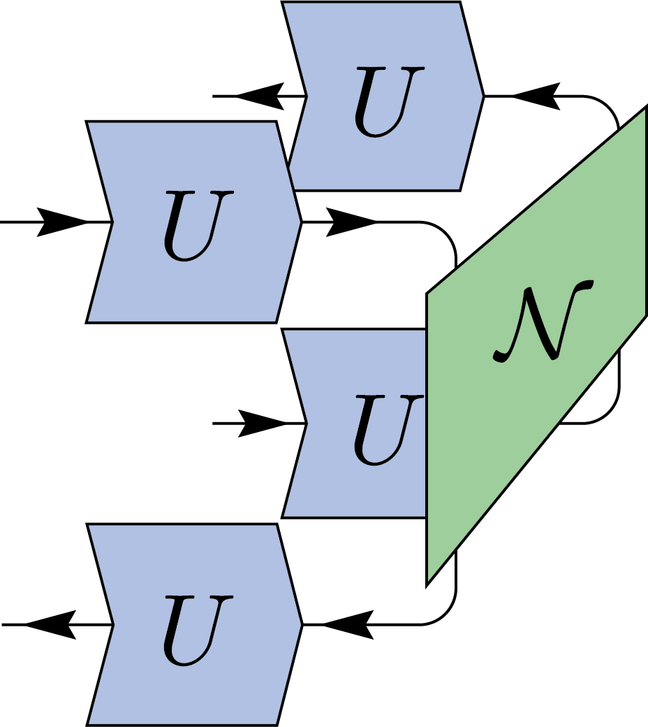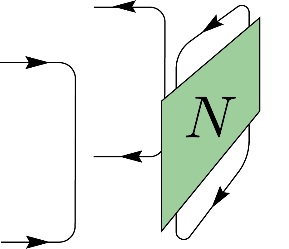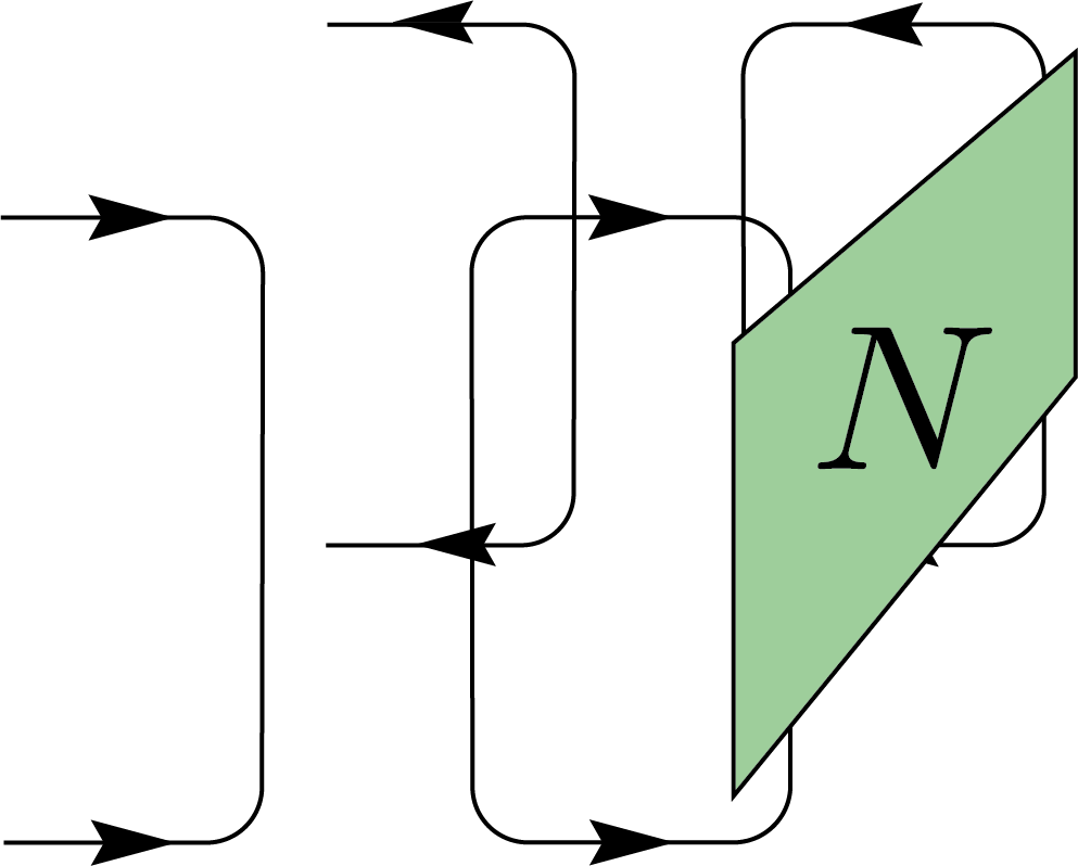\] By contracting the output register with EPR states, we obtain a similar twirling identity for two-register states \(N\). This process is typically used when studying entanglement between two parties, Alice and Bob. We can interpret this twirling as Alice and Bob applying a random unitary (LOCC) to each side of their system.

\( \displaystyle\int\) \(=\) \(\displaystyle\int\) \(=\) \(\displaystyle\int\) \(=\frac{1}{d^2-1}\Biggl(\) \(+\) \(\Biggl)+\frac{1}{d-d^3}\Biggl(\) \(+\) \(\Biggl)\)

The result is a Werner state (here including the normalization factor \(d\)): \[ (1-\lambda)\ket{\mathrm{EPR}}\bra{\mathrm{EPR}} + \lambda\frac{\mathbb{I}}{d^2}, \] where \[ \lambda = \frac{d^2 - \langle N \rangle_{\ket{\mathrm{EPR}}}}{d^2 - 1}. \]