Figures

Figure 1: Depth-integrated total transport of the model mean circulation. The mean circulation is found over one year. The contour interval is 10 Sverdrups.

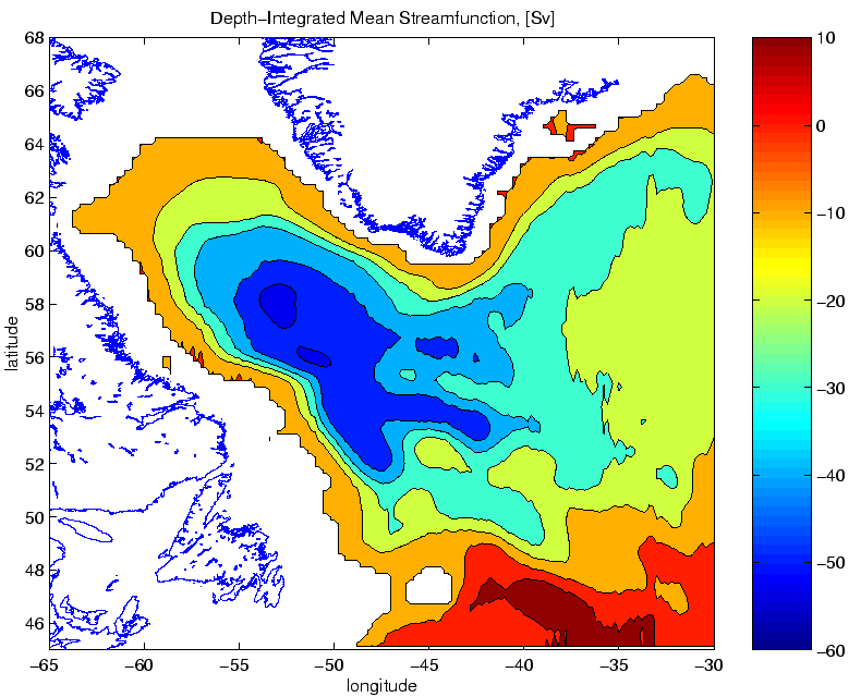Figure 2: Geostrophic height contours of the mean model circulation at 700 meters depth. The contour interval is 2 centimeters of geostrophic height.

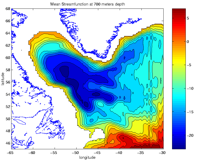Figure 3: Difference in model values between September 1997 and October 1996 as a function of depth.

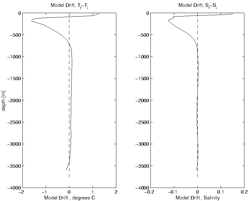Figure 4: 10-day average model temperature profile for March 1-10, 1997, along the AR7W WOCE cross-section. The model section includes 24 gridpoints. The observed data is on the following page.

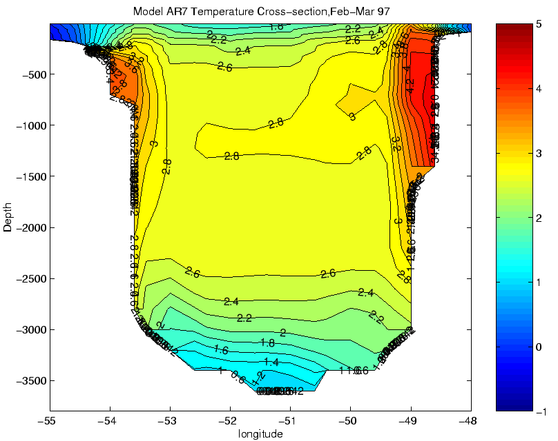Figure 5: Observed temperature profile for Feb 26-Mar 6, 1997, along the AR7W WOCE cross-section (courtesy R. Pickart).

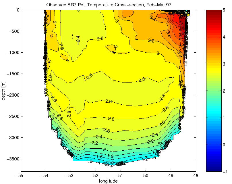Figure 6: 10-day average model salinity profile for March 1-10, 1997, along the AR7W WOCE cross-section. The observed data is on the following page.

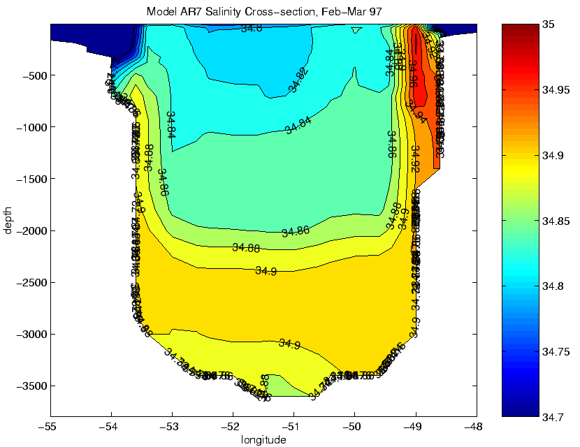Figure 7: Observed salinity profile for Feb 26-Mar 6, 1997, along the AR7W WOCE cross-section (courtesy R. Pickart). The section is comprised of 37 stations.

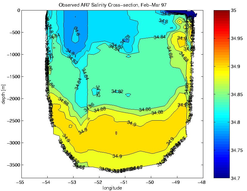Figure 8: 10-day average model temperature profile for June 8-17, 1997, along the AR7W WOCE cross-section. The observed data is on the following page.

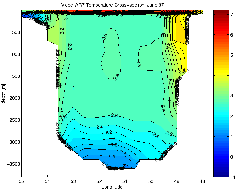Figure 9: Observed temperature profile for June 11-18, 1995, along the AR7W WOCE cross-section (courtesy J. Lazier). The section is comprised of 24 stations.

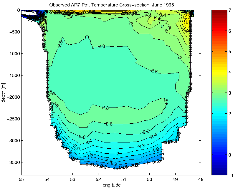Figure 10: 10-day average model salinity profile for June 8-17, 1997, along the AR7W WOCE cross-section. The observed data is on the following page.

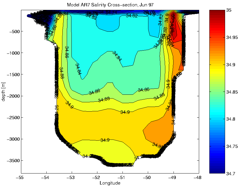Figure 11: Observed salinity profile for June 11-18, 1995, along the AR7W WOCE cross-section (courtesy J. Lazier).

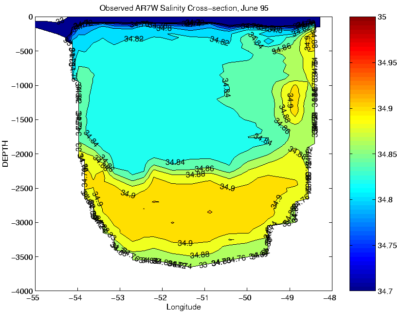Figure 12: Model temperature profile at Bravo mooring site ( $56.2^{\circ } N,-51.0 ^{\circ } E$) for 8 months of the winter convective season (Nov-May). The observed profile was published by Lab Sea Group, 1998.

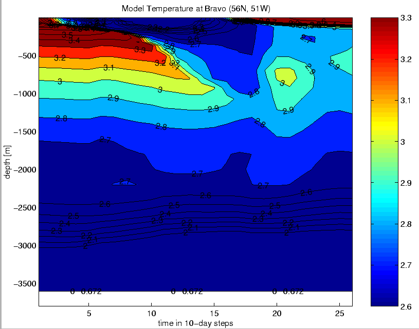Figure 13: One sample temperature profile from a PALACE float (solid) versus the GCM (dashed) for four different times within the convective region.

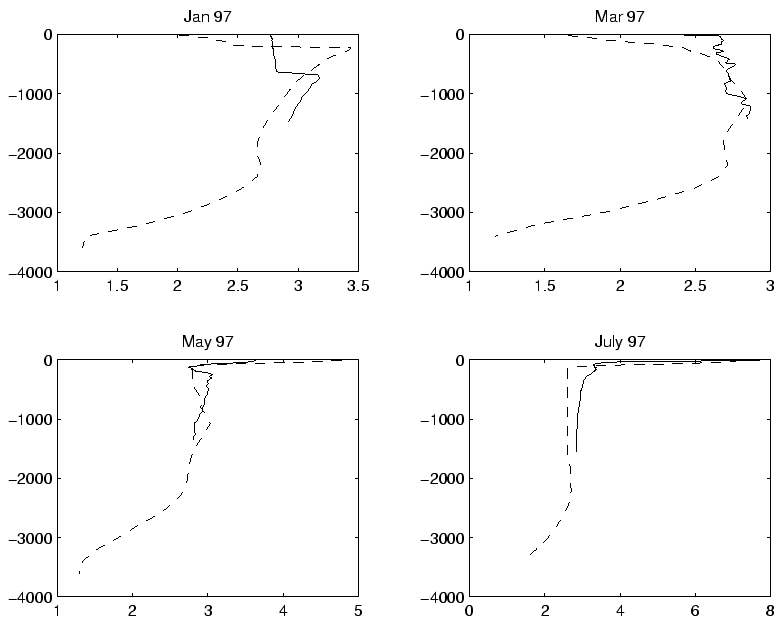Figure 14: One sample salinity profile from a PALACE float (solid) versus the GCM (dashed) for four different times within the convective region.

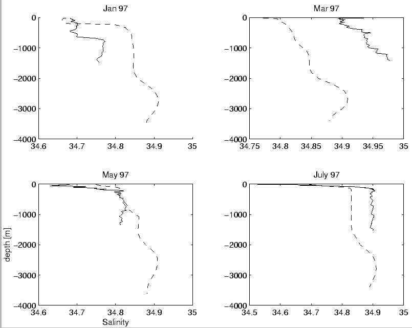Figure 15: Sea surface height variance computed from one year of 10-day average model output. The maximum value is $499.5 cm^2$. The Topex/Poseidon estimates of SSH Variance are on the following page.

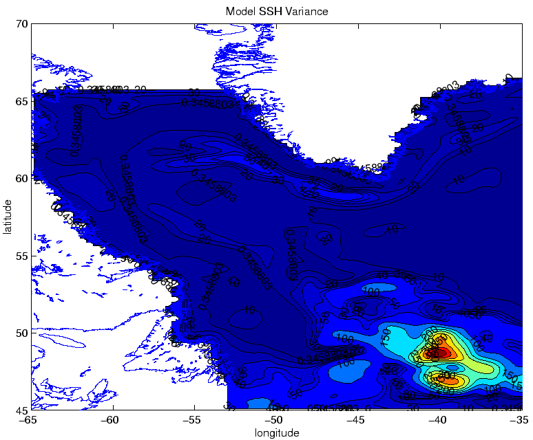Figure 16: Even tracks of SSH variance from one year of raw T/P data and one year of model 10-day averages. Model data was interpolated to the satellite tracks using a simple ``closest neighbor'' approach.

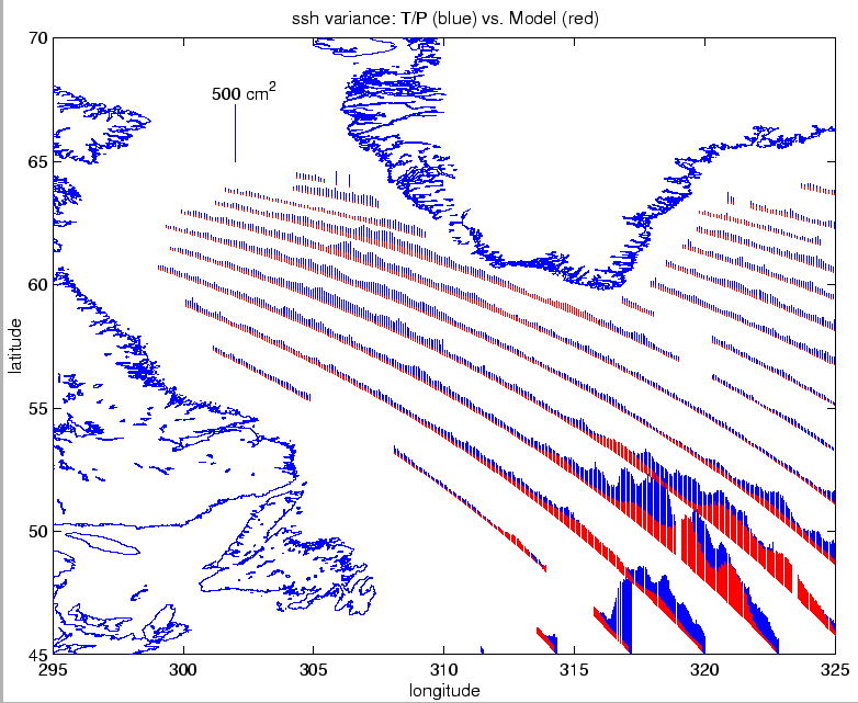Figure 17: Odd tracks of SSH variance. The Topex/Poseidon variance is larger than the model variance in 95% of the points.

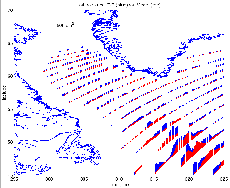Figure 18: Frequency spectra from 2 T/P points (solid, dotted) at a crossover point for 6 years duration and frequecy spectrum from one model point (dashed) of one year of one day average values. A 6-point Danielle window stabilized the spectra and consequently shortened the bandwidth slightly.

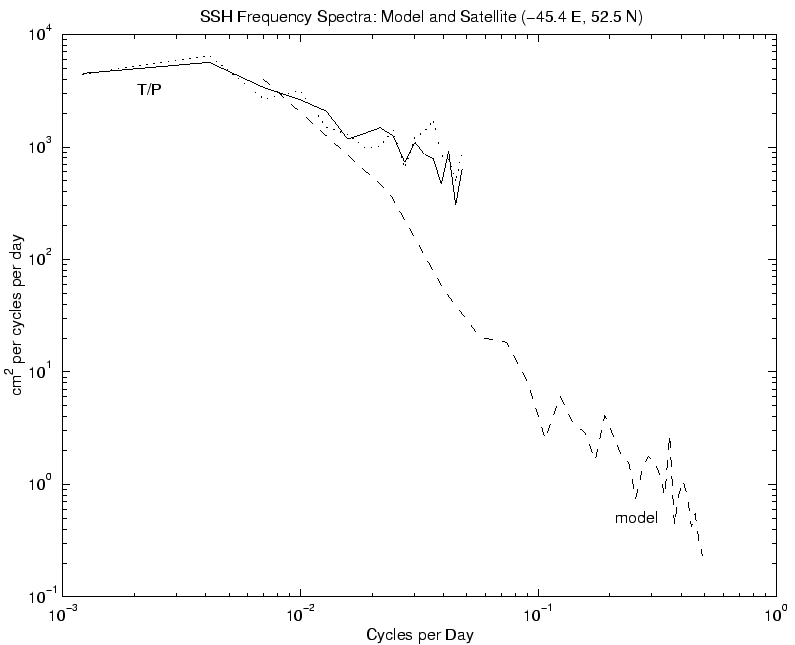Figure 19: Frequency spectra computed using the same process as the previous figure. 2 T/P crossover points versus one model point (dashed).

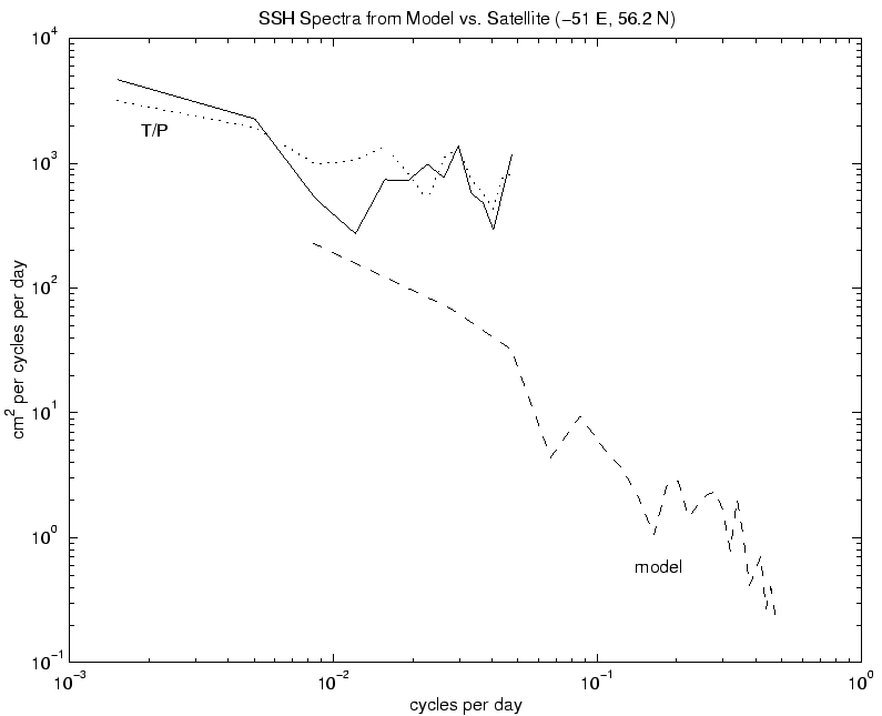Figure 20: Average surface geostrophic eddy kinetic energy for one year The energy was computed from the sea surface pressure field.

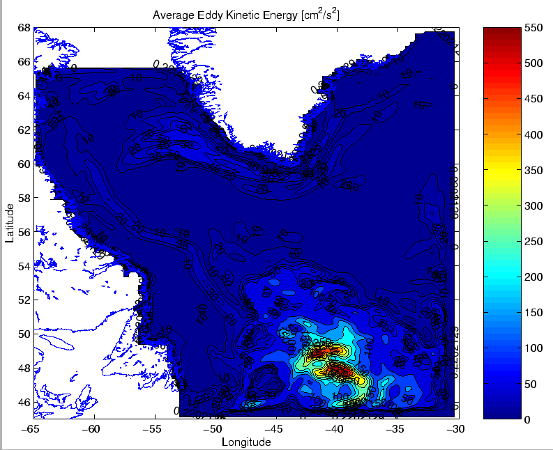Figure 21: Left Side: Observed $K_{E}$ at 4 depths (circles) and the extrapolated profile from a Gauss-Markov fit at site 91 ( $57 \deg N, -51.1 \deg E$). Right side: Model $K_{E}$ profile. Notice the change in scales of one or two orders of magnitude.

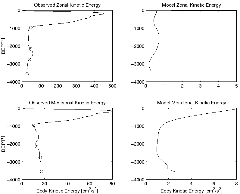Figure 22: Model velocity timeseries as a function of depth for one year from 10-day time averages at site 91 ( $57 ^{\circ } N, -51.6 ^{\circ } E$). Velocities are indicated by displacement from the dotted line. Maximum velocities are approximately 20 cm/s.

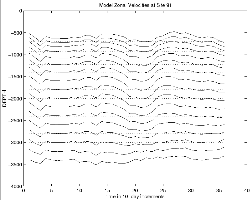Figure 23: A comparison between observed eddy kinetic energy at 3 depths (circles), the extrapolated kinetic energy profile from a Gauss-Markov fit (dashed), and the model kinetic energy profile (solid) at site 89 ( 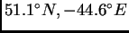$51.1 ^{\circ } N, -44.6 ^{\circ } E$). An 'X' marks the surface intensified energy of the uppermost model gridpoint.

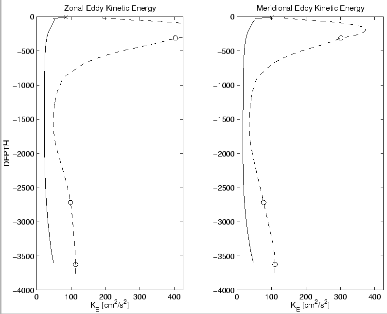Figure 24: The ratio of eddy kinetic energy at the ocean bottom to 1500 meters. Results are shown here for all depths greater than 1500 meters.