1.022 Final Project:¶

Modeling the nation-wide spread of COVID-19¶

We have carefully crafted the final project to provide you with an opportunity to gain experience dealing with a real-world application of networks. As a particular case of interest, we will design, evaluate, and refine an epidemic model to predict the total number of covid cases in the US over time.

1. Collecting and plotting data on covid cases¶

As the first step, we collect historic and current data on total number of covid cases across the nation via nytimes covid-19 bot.

Run the code below to:¶

get the daily record of the cumulative counts of covid cases at the state level
process the gathered data to get daily and weekly counts of new cases at both state and national levels

import numpy as np
import pandas as pd
import itertools
import pickle
from scipy.linalg import norm
from scipy.linalg import expm
from scipy.optimize import minimize
import os
from timeit import default_timer as timer
import matplotlib.pyplot as plt
plt.style.use('seaborn')
import nytimes

# some basic national demographics (including population of each
# state to be used in normalization of covid counts)
state_geo = pd.read_csv('states_demographics.csv',\
                    dtype={'state_fips':str}).set_index('state_id')

raw_states_df, _ = nytimes.get_nyt_data()
state_cases = nytimes.convert_state_df_to_ts(\
        raw_states_df, quantity = 'cases').drop(columns=['state']).T
state_cases.index = pd.to_datetime(state_cases.index)
state_cases = state_cases[state_geo['state_name']]
state_cases.columns = state_geo.index.copy()
state_cases_daily = state_cases.diff()
t_last_na = state_cases_daily.isna().any(axis=1).cumsum().idxmax()
state_cases_daily.dropna(inplace=True)
state_cases_weekly = 7*state_cases_daily.resample(\
                        '7D').mean().divide(state_geo['population'])

cumul_offset = state_cases.loc[t_last_na].divide(state_geo['population'])
state_cases_cumulative = state_cases_weekly.cumsum() + cumul_offset

nation_cases_daily = state_cases_daily.sum(axis=1)
nation_cases_weekly = 7*nation_cases_daily.resample('7D').mean()\
                                       /state_geo['population'].sum()
nation_cumul_offset = state_cases.loc[t_last_na].sum()\
                                       /state_geo['population'].sum()
nation_cases_cumulative = nation_cases_weekly.cumsum()\
                                                + nation_cumul_offset

The processed data that we will use in our design is weekly new covid cases and cumulative number of cases, gathered in DataFrames state_cases_weekly, state_cases_cumulative for state level data, and as two Series nation_cases_weekly ,nation_cases_cumulative for the country level data, all starting at March 18 and having 7D frequency.

Here is a snapshot from state level weekly count of new covid cases (state_cases_weekly):

state_id	AL	AZ	AR	CA
2020-03-18	0.000041	0.000042	0.000069	0.000048
2020-03-25	0.000154	0.000134	0.000110	0.000150
2020-04-01	0.000244	0.000176	0.000143	0.000227

Both weekly and cumulative number of cases are normalized by the population of their states for the state level data, and by US population for the national level data

From now on and in the rest of this manuscript, number of cases by default refers to their values after normalization ( a number between 0 and 1), unless explicitly stated otherwise.

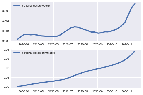
Task 1.1

Use the collected data to plot: (i) weekly count of new covid cases in the US, and (ii) cumulative number of cases in the US.

fig, axes = plt.subplots(2,1)
iter_axes = itertools.cycle(fig.axes)

ax = next(iter_axes)
ax.cla()
ax.plot(nation_cases_weekly,\
        label='national cases weekly', linewidth=4); ax.legend()

ax = next(iter_axes)
ax.cla()
ax.plot(nation_cases_cumulative,\
        label='national cases cumulative', linewidth=4); ax.legend()

2. Fitting a basic SIR model to the covid data¶

Task 2.1

Show that in the basic SIR model, so long as the size of the infection is very small (e.g., early stages of the spread), we can approximate the dynamics of the spread by:

\[\begin{split}\begin{align*}\dot{S}(t) &=-\beta~I(t)\\ \dot{I}(t) &= (\beta - \gamma)~I(t) \end{align*}\end{split}\]

Use this simplified dynamics to show that:

\[S(t) \approx S(0) -\frac{\beta}{\beta-\gamma}(e^{(\beta~-~\gamma)t}-1)~I(0)\]

Observe the three identical quantities: the (normalized) cumulative number of cases at time \(t\) \(\equiv\) \(1-S(t)\) \(\equiv\) the fraction of the population that are either infected or recovered/removed by time \(t\) (IR population).

The function SIR implemented below simulates \(T\) steps of the SIR model based on the above approximation.

Inputs to the SIR function:

beta: the average infection/contact rate in the population
gamma: the average recovery rate for each infected case
IR_init: the initial size of infected-or-recovered/removed cases (\(I(0)+R(0)\))
I_init: the initial size of the infected cases (\(I(0)\))
T: the number of time steps to run the model. Each step here represents a week (7D)

The function will then output:

IR_1_to_T: The cumulative number of covid cases at \(t= 1, \ldots, T\) as predicted by the model

def SIR(beta, gamma, IR_init, I_init, T):
     IR_1_to_T = (np.exp((beta-gamma)*np.arange(1,T+1))-1)*\
                                 beta*I_init/(beta-gamma) + IR_init
     return IR_1_to_T

The next step is to tune the parameters of the model, namely \(\beta\) and \(\gamma\) using the data we prepared earlier.

Let us choose March 18, as t=0. Use the cumulative number of cases in the US on March 18 (top entry of nation_cases_cumulative) as IR_init. We further assume I_init = IR_init (i.e., \(\small R(0)\approx0\)). This can be justified noting that on March 18 the spread was at its very early stages, hence only a small fraction of infected cases had recovered by then.

The goal is to choose \(\beta\) and \(\gamma\) such that number of cases as predicted by the model stays close to that observed from data. The standard approach is to choose a loss function, measuring how off the predictions are from observed data, and then tune the parameters such that they minimize the loss.

Here, we search for \(\beta\) and \(\gamma\) minimizing the sum of the squares of prediction errors for the US cumulative number of cases, over a period of \(T=16\) weeks (from March 25 to July 08)

\[{\underset{\beta, \gamma}{\rm minimize}} \sum_{t=1}^T \big(IR_{\rm predicted}(t)-IR_{\rm data}(t)\big)^2\]

Note that March 18 data is already used in initializing the model (IR_init).

Here is the code implementing this loss function:

def SIR_LOSS(params, IR_init, I_init, observed_cumulative_cases):
    beta, gamma = params
    T = len(observed_cumulative_cases)
    predicted_IR = SIR(beta, gamma, IR_init, I_init, T)
    loss = norm(observed_cumulative_cases-predicted_IR)**2
    return loss

Inputs and outputs to SIR_LOSS function:

params: to pass the values of \(\beta\) and \(\gamma\) to the loss function.
IR_init: The initial size of the infected-or-recovered cases (\(I(0)+R(0)\))
I_init: The initial size of the infected cases (\(I(0)\))
observed_cumulative_cases: The cumulative number of covid cases in the US as observed from data

The function will then output:

loss: The sum of squares of prediction errors in cumulative number of cases in the US as predicted by the model

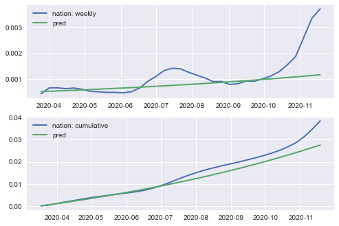
Task 2.2

Use the function minimize from scipy.optimize package to find values of \(\beta\) and \(\gamma\) minimizing the loss function SIR_LOSS for a period of \(T=16\) weeks from March 25 to July 08. (Choose data from nation_cases_cumulative for this period to pass as observed_cumulative_cases to the loss function)
Pass the values \(\beta\) and \(\gamma\) you obtain to the SIR function to predict the cumulative number of covid cases in the US for 36 weeks starting from March 18.
Plot the predictions together with observed data for both (i) cumulative number of cases and (ii) weekly new cases ( use np.diff() to obtain the latter)

n_train = 16
IR_init = I_init = nation_cases_cumulative[0]
observed_cumul_cases = nation_cases_cumulative[1:n_train+1].values

params_init = [0.1,0.01]
res = minimize(SIR_LOSS, params_init,\
                 args = (IR_init, I_init, observed_cumul_cases))
beta_SIR, gamma_SIR = res['x']
print('success:{}, beta: {:.3f}, gamma:{:.3f}'.format(\
                                res['success'], beta_SIR, gamma_SIR))

success:True, beta: 2.984, gamma:2.959

# pred over entire data/visualize
T = len(nation_cases_cumulative[1:])
predicted_cumul_cases = SIR(beta_SIR, gamma_SIR,\
         nation_cases_cumulative[0], nation_cases_cumulative[0], T)
predicted_cumul_cases = \
        np.append(nation_cases_cumulative[0],predicted_cumul_cases)
predicted_weekly_cases = np.diff(predicted_cumul_cases)

fig, axes = plt.subplots(2,1)
iter_axes = itertools.cycle(fig.axes)
ax = next(iter_axes); ax.cla()
ax.plot(nation_cases_weekly[1:], \
            label= '{}: weekly'.format('nation'), linewidth=2)
ax.legend()
ax.plot(nation_cases_weekly.index[1:],\
             predicted_weekly_cases, label='pred', linewidth=2)
ax.legend()
ax = next(iter_axes); ax.cla()
ax.plot(nation_cases_cumulative,\
         label='{}: cumulative'.format('nation'), linewidth=2)
ax.legend()
ax.plot(nation_cases_cumulative.index,\
         predicted_cumul_cases, label='pred', linewidth=2)
ax.legend()

3. Refining the design by incorporating SafeGraph mobility data¶

The performance of the basic SIR design reveals the necessity to account for the behavioral dynamics of a population dealing with a pandemic, in order to have more reliable predictions. In this part, we refine our initial design by incorporating mobility data provided by SafeGraph in order to cope with changes in inter-state mobility across the US in the covid era.

To save you time, we have already processed and trimmed daily US mobility data starting from January 1st up until now. The end result accessible via ‘interstate_mobility.pickle’ is a dictionary providing weekly averaged inter-state mobility data for the period of January 1 - November 11 (a total of 46 weeks). Each item in the dictionary is a tuple (date, df), where:

df.loc[st1, st2] counts the number of devices from state st1 who visited state st2, averaged over the week starting from date.
diagonal entries of df count the number of devices not leaving their home state, averaged over the same week.

with open('interstate_mobility.pickle', 'rb') as f_handle:
   interstate_mobility_weekly = pickle.load(f_handle)

# let's look inside
date = pd.Timestamp('2020-03-18')
pd.options.display.float_format = '{:.2f}'.format
display(interstate_mobility_weekly[date].iloc[:4,:6])

	AL	AZ	AR	CA	CO	CT
state_id
AL	763322.43	233.57	488.29	529.57	235.57	45.00
AZ	185.14	604555.00	229.14	7336.14	1219.43	49.00
AR	481.86	229.57	399036.29	342.00	240.57	9.43
CA	553.86	8497.00	636.29	2385812.14	1887.86	209.14

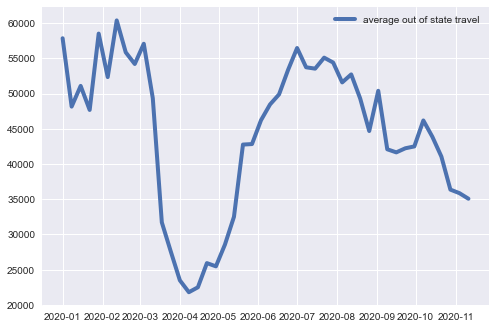
Task 3.1

Calculate and plot average out-of-state travel by adding up off-diagonal entries in each DataFrame and normalizing the result by the number of states. Is there any noticable fluctuations in travel volume in response to covid? Summarize your observations from the plot (max. 5 lines).

avg_inflow ={}
for date, df in interstate_mobility_weekly.items():
   avg_inflow[date] = (np.sum(df.values) - np.trace(df))/df.shape[0]

avg_inflow = pd.Series(avg_inflow)
plt.plot(avg_inflow,\
                   label='average out of state travel', linewidth=4)
plt.legend()

A networked SIR model with time-varying inter-state mobility¶

This is an enhanced version of the networked SIS model discussed in the lecture, capturing the effect of changes in inter-state mobility over time.

The population of any state \(j\) at time \(t\) is compromised of (i) those who have travelled to state \(j\) from other states, and (ii) those whose home state is \(j\) and have not travelled elsewhere. We use \(n_{ij}(t)\) to denote the number of individuals with home state \(i\) who are in state \(j\) at time \(t\). The infected and susciptible populations currently at state \(j\) are then \(\sum_{i=1}^{n}n_{ij}(t)I_i(t)\) and \(\sum_{i=1}^{n}n_{ij}(t)S_i(t)\). Normalized sizes become:

\[\begin{split}\begin{align} {\hat I}_j(t)=&\sum_{i=1}^{n}c_{ij}(t)I_i(t)\\ {\hat S}_j(t)=&\sum_{i=1}^{n}c_{ij}(t)S_i(t), \end{align}\end{split}\]

where \(c_{ij}(t):=\frac{n_{ij}(t)}{\sum_{i=1}^{n}n_{ij}(t)}\). Observe that \(c_{ij}(t)\) normalizes the inflow to state \(j\) to 1. In other words, matrix \(C(t)=[c_{ij}(t)]\) is column-stochastic.

The size of new infections is \(\beta_j {\hat I}_j(t){\hat S}_j(t)\). During the early stages, we can use the first order approximation \(\beta_j {\hat I}_j(t)\) for the size of new infections, out of which the share of travellers from state \(i\) is \(\beta_j {\hat I}_j(t) n_{ij}(t)\) newly infected individuals, taking the virus with themselves back to their home state \(i\).

The aggregate size of new cases among residents of state \({\bf i}\) thus becomes \(\sum_{j=1}^{n}\beta_j {\hat I}_j(t) n_{ij}(t)\), or equivalently \(\sum_{i=j}^{n}\beta_j {\hat I}_j(t) \rho_{ij}(t)\), when normalized with their population size \(\sum_{j=1}^{n} n_{ij}(t)\). Note that, here \(\rho_{ij}(t) :=\frac{n_{ij}(t)}{\sum_{j=1}^{n}n_{ij}(t)}\). That is, \(\rho_{ij}(t)\) normalizes the outflow from state \(i\) to 1. In other words, matrix \({\rm P}(t)=[\rho_{ij}(t)]\) is row-stochastic. The continuous-time approximate update rule for state \(i\) then becomes:

\[\begin{split}\begin{align*} \dot{S}_i{(t)} &= -\sum_{j=1}^{n}\rho_{ij}(t)\beta_j {\hat I}_j(t)\\ \dot{I}_i(t)&=\sum_{j=1}^{n}\rho_{ij}(t)\beta_j {\hat I}_j(t) - \gamma I_i(t) \end{align*}\end{split}\]

Task 3.2

Verify that the dynamics described above can be written in the following compact form:

\[\begin{split}\begin{align*} \dot{S}(t) &= -{\rm P}(t)~{\rm diag}(\beta)~C^T(t)~I(t)\\ \dot{I}(t) &= \big({\rm P}(t)~{\rm diag}(\beta)~C^T(t)-\gamma~{\rm Id.}\big)~I(t) \end{align*}\end{split}\]

where \({\rm P}(t) = [\rho_{ij}(t)]\) and \(C(t)=[c_{ij}(t)]\) are row-stochastic and column-stochastic versions of the inter-state mobility matrix, respectively.

Can you justify the use of different contact rates, but a common recovery rate for different states?

The solution to the above continuous-time dynamics can be written as:

\[\begin{split}\begin{align*} I(t) &= e^{\int_0^{t}\big({\rm P}(\tau)~{\rm diag}(\beta)~C^T(\tau)-\gamma~{\rm Id.}\big)d\tau}~I(0)\\ S(t) &= S(0) -\int_0^{t} {\rm P}(\tau)~{\rm diag}(\beta)~C^T(\tau)~I(\tau)~d\tau \end{align*}\end{split}\]

where \({\rm Id.}\) stands for the identity matrix.

We use the following discrete-time approximation in our analysis:

\[\begin{split}\begin{align*} I(t+1)&=e^{\sum_{\tau=0}^{t}\big({\rm P}(\tau)~{\rm diag}(\beta)~C^T(\tau)-\gamma~{\rm Id.}\big)}~I(0)\\ S(t+1) &= S(0) - \sum_{\tau=0}^{t} {\rm P}(\tau)~{\rm diag}(\beta)~C^T(\tau)~I(\tau) \end{align*}\end{split}\]

The function Networked_SIR implemented below simulates \(T\) steps of our networked SIR model based on the above approximation.

Inputs to the Networked_SIR function:

beta: 1D array whose elements are the infection rates of different states
gamma: the common recovery rate
IR_init: 1D array represeting the initial size of the IR population in each state
I_init: 1D array represeting the initial size of the infected population in each state
C_matrices: \(T\times n_{\rm states}\times n_{\rm states}\) array. C_matrices[t] represents inter-state mobility matrix with inflows normalized to 1 (column sum=1) at time \(t\) for \(t=0,1,\ldots, T-1\)
P_matrices: \(T\times n_{\rm states}\times n_{\rm states}\) array. P_matrices[t] represents inter-state mobility matrix with outflows normalized to 1 (row sum=1) at time \(t\) for \(t=0,1,\ldots, T-1\)
T: the number of time steps to simulate the model and make predictions for \(t=1,\ldots, T\). Each step again represents a week (7D)

The function will then output:

A tuple (IR, I) of two \(T\times n_{\rm states}\) arrays giving model predictions for size of IR and I populations in each state for \(t= 1, \ldots, T\)

def Networked_SIR(beta, gamma, IR_init, I_init,\
                                    C_matrices, P_matrices):
    n_states = len(I_init)
    T = len(C_matrices)

    I = np.zeros((T+1,n_states))
    IR = np.zeros((T+1,n_states))
    I[0], IR[0] = I_init.copy(), IR_init.copy()
    # I[0], IR[0] = I_init[:,0].copy(), IR_init[:,0].copy()
    for t in range(T):
        P_beta_CT_t = P_matrices[t].dot(\
                       np.diag(beta).dot(C_matrices[t].T))
        I[t+1] = np.dot(expm(\
                       P_beta_CT_t - gamma*np.eye(n_states)),I[t])
        IR[t+1] = IR[t] + np.dot(P_beta_CT_t,I[t])
    return IR[1:], I[1:]

Here, we search for \(\beta = [\beta_1,\ldots,\beta_{n_{\rm states}}]\) and \(\gamma\) minimizing the following loss:

\[{\underset{\beta, \gamma}{\rm minimize}} \sum_{t=1}^T \sum_{i=1}^{n_{\rm states}}\frac{\big(\text{cumulative cases from data}(i,t) - \text{predicted cumulative cases}(i,t)\big)^2}{n_{\rm states}\times T}\]

This is the average of the losses of individual states’ predictions for the raw number of cases and not the normalized counts (can you guess why we do not use normalized counts here?).

Here is the code implementing this loss function:

def Networked_SIR_LOSS(params, IR_init, I_init,\
                    C_matrices, P_matrices, observed_cumul_cases):
    beta, gamma = params[:-1], params[-1]
    n_states = len(I_init)
    T = len(P_matrices)

    predicted_IR, predicted_I = Networked_SIR(beta, gamma,\
                         IR_init, I_init, C_matrices, P_matrices)

    error_in_cumul_cases = (observed_cumul_cases-predicted_IR)\
                                    *state_geo['population'].values
    # normalizing the error with number of states and T.
    # The devision by 1000 is just for the error not to blow up!
    loss = norm(error_in_cumul_cases/(n_states*T*1000))**2
    return loss

Inputs and outputs to Networked_SIR_LOSS function:

params: 1D array to pass model parameters \(\beta\) and \(\gamma\) to the loss function.
IR_init: the initial size of infected-or-recovered cases for each state - I_init: the initial size of infected cases for each state
C_matrices: \(T\times n_{\rm states}\times n_{\rm states}\) array. C_matrices[t] represents inter-state mobility matrix with inflows normalized to 1 (column sum=1) at time \(t\) for \(t=0,1,\ldots, T-1\)
P_matrices: \(T\times n_{\rm states}\times n_{\rm states}\) array. P_matrices[t] represents inter-state mobility matrix with outflows normalized to 1 (row sum=1) at time \(t\) for \(t=0,1,\ldots, T-1\)
observed_cumul_cases: \(T\times n_{\rm states}\) array passing the observed cumulative count of covid cases in each state for \(t=1,\ldots, T\).

Note that we still pass the normalized value of observed_cumul_cases to the loss function. The conversion to raw numbers is implemented inside the function.

The function will then output:

loss: The sum of squares of prediction errors in cumulative case counts at state level, averaged over all the states

Task 3.3

Use the function minimize from scipy.optimize package to find values of \(\beta=[\beta_1,\ldots,\beta_{n}]\) and \(\gamma\) minimizing the loss function Networked_SIR_LOSS over a period of \(T=16\) weeks, from March 25 to July 08. (Choose data from state_cases_cumulative for this period to pass as observed_cumul_cases to the loss function)
make a bar plot of \(\beta\) values versus their state ids (use state_geo.index for state ids)
Pass the values obtained for \(\beta\) and \(\gamma\) to Networked_SIR function and use its output to predict the cumulative number of covid cases in the US for 36 weeks starting from March 18.
Plot the predictions together with observed data for both (i) cumulative number of cases and (ii) weekly new cases ( use np.diff() to obtain the latter)

t_init = state_cases_cumulative.index[0]
datelist = avg_inflow[t_init:].index
C_matrices = np.array([interstate_mobility_weekly[date].div(\
    interstate_mobility_weekly[date].sum(axis=0), axis=1).values\
                                              for date in datelist])
P_matrices = np.array([interstate_mobility_weekly[date].div(\
    interstate_mobility_weekly[date].sum(axis=1), axis=0).values\
                                              for date in datelist])

IR_init = I_init = state_cases_cumulative.head(1).values[0]
n_states = len(I_init)
beta, gamma = beta_SIR*np.ones(n_states), gamma_SIR
params_init = np.append(beta,gamma)